Understanding Weibull Analysis
The two-parameter Weibull is by far the most widely used distribution for life data analysis:

Where:
t≥0, β≥0 and η>0. Here, β and η are shape and scale (characteristic life) parameters of the distribution.
Because two-parameter Weibull distribution effectively analyses the life data from burn-in (infant mortality), useful life and wear-out periods, it can be used in increasing, constant and decreasing failure rate situations.
The first parameter defining the Weibull probability plot is the slope, beta (β), which is also known as the shape parameter because it determines which member of the Weibull family of distributions best fits or describes the data. The second parameter is the characteristic life, eta (η),which is also known as the scale parameter because it defines where the bulk of the distribution lies. The parameters β and η are estimated from the life data, which are always positive values. After Weibull analysis is completed, the Weibull probability plot visually indicates the slope and the goodness of fit.
A three-parameter Weibull distribution is also widely used. The third parameter, location, is a constant value that is added to or subtracted from the time variable, . For additional information, refer to page 7-15. |
The Weibull hazard function or failure rate depends upon the value of β. Because the β value indicates whether newer or older parts are more likely to fail, the Weibull hazard function can represent different parts of the bathtub curve:
• Infant Mortality. In electronics and manufacturing, infant mortality refers to a higher probability of failure at the start of the service life. When the β value is less than 1.0, the Weibull probability plot indicates that newer parts are more likely to fail during normal usage, which is known as a decreasing instantaneous failure rate. To end infant mortality in electronic and mechanical systems with high failure rates, manufacturers provide production acceptance tests, “burn-in” and environmental stress screenings prior to delivering such systems to customers. Providing that the part survives infant mortality, its failure rate should decrease, and its reliability should increase. In this case, because such parts tend to fail early in life, old parts are considered better than new parts. Overhaul of parts experiencing high infant mortality is generally not appropriate.
• Random Failures. Assuming that the Weibull probability plot is based on a single failure mode, a β value of 1.0 indicates that the failure rate is constant or independent of time. This means that of those parts that survive to time t, a constant percentage will fail in the next unit of time, which is known as a constant hazard rate or instantaneous failure rate. This makes the Weibull probability plot identical to the exponential distribution. Because old parts are assumed to be as good as new parts, overhaul is generally not appropriate. The only way to increase reliability for components or systems that experience random failures is by redesigning them.
• Early Wear-out. Unexpected failures during the design life are often due to mechanical problems. When the β value is greater than 1.0 but less than 4.0, overhauls or part replacements at low B-lives may be cost effective. B-lives indicate the ages at which given percentages of the population are expected to fail. For example, the B-1 life is the age at which 1 percent of the population is expected to fail, and the B-10 life is the age at which 10 percent of the population is expected to fail. Reliability and cost performance for parts experiencing early wear-out may be improved by optimizing the preventative maintenance schedule.
• Rapid Wear-out. Although a β value greater than 4.0 within the design life of a part is a major concern, most Weibull probability plots with steep slopes have a safe period within which the probability of failure is negligible, and the onset of failure occurs beyond the design life. The steeper the slope, the smaller variation in the times to failure and the more predictable the results. For parts that have significant failures, overhauls and inspections may be cost effective. Because scheduled maintenance can be costly, it is usually only considered when older parts are more likely to wear out and fail, which is known as an increasing instantaneous failure rate.
Because different slopes imply different failure classes, the Weibull probability plot provides clues about what may be causing the failures. Table 7-1 lists the failure causes that are most likely for each failure class.
β value | Class | Description |
|---|---|---|
β<1.0 | Infant Mortality | When β < 1.0, failures tend to be due to: • Inadequate burn-in or stress screening. • Quality problems in components. • Quality problems in manufacturing. • Improper installation, setup or use. • Problems in rework/refurbishment. |
β=1.0 | Random Failures | When β = 1.0, failures tend to be due to: • Human error during maintenance. • Induced rather than inherent failures. • Accidents and natural disasters (foreign objects, lighting strikes, wind damage, etc.). |
β>1.0 and <4.0 | Early Wear-out | When β > 1.0 and < 4.0, failures tend to be due to such problems as: • Low cycle fatigue. • Bearing failures. • Corrosion/erosion. • Manufacturing process. |
β>4.0 | Rapid Wear-out | When β> 4.0, failures tend to be due to rapid wear-out associated with old age or: • Inherent property limitations of materials (such as ceramic being brittle). • Severe problems in manufacturing process. • Minor variability in manufacturing or in material. |
Statisticians, mathematicians and engineers have formulated statistical distributions to mathematically model or represent certain behaviours. Compared to other statistical distributions, the Weibull distribution fits a much broader range of life data. The Weibull probability density function (pdf) is the mathematical function that describes the fitted curve over the data. The pdf is represented either mathematically or on a plot where the X-axis represents times. Different members of the Weibull family have widely different shaped pdfs. The cumulative density function (cdf) is the area under the curve of the pdf. The cdf for the Weibull distribution is given by:

Where:
η represents the characteristic life (scale parameter).
β represents the slope (shape parameter).
The cdf gives the probability of failure within time, t. The parameters η and β are estimated from the failure times. If the failure data comes from a Weibull distribution, the values of η and β can be plugged in the cdf formula to find the fraction of parts expected to fail within a certain time.
Characteristic life, η, and the Mean Time To Failure (MTTF) are related. The characteristic life shows the point in the life of the part or system where the failure probability is independent of the parameters of the failure distribution. For all Weibull distributions, η is defined as the age at which 63.2 percent of the units can be expected to have failed.
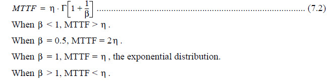
For β= 1, MTTF and are equal. The relationship between MTTF and η is gamma function:
Although Professor Weibull originally proposed using the mean or average value to plot MTTF values on the Y-axis of Weibull probability plots, the standard engineering method is now to rank the life data by the median value of the failure times. Table 7-2 displays a Median Ranks table (50%) for a sample size of 10, which was generated using Leonard Johnson’s Rank formula.
Because non-symmetrical distributions are so common in life data, median rank values are slightly more accurate than mean values. Once β and η are known, the probability of failure at any time can easily be calculated.
Rank Order | 1 | 2 | 3 | 4 | 5 | 6 | 7 | 8 | 9 | 10 |
|---|---|---|---|---|---|---|---|---|---|---|
1 | 50.00 | 29.29 | 20.63 | 15.91 | 12.94 | 10.91 | 9.43 | 8.30 | 7.41 | 6.70 |
2 | 70.71 | 50.00 | 38.57 | 31.38 | 26.44 | 22.85 | 20.11 | 17.96 | 16.23 | |
3 | 79.37 | 61.43 | 50.00 | 42.14 | 36.41 | 32.05 | 28.62 | 25.86 | ||
4 | 84.09 | 68.62 | 57.86 | 50.00 | 44.02 | 39.31 | 35.51 | |||
5 | 87.06 | 73.56 | 63.59 | 55.98 | 50.00 | 45.17 | ||||
6 | 89.09 | 77.15 | 67.95 | 60.69 | 54.83 | |||||
7 | 90.57 | 79.89 | 71.38 | 64.49 | ||||||
8 | 91.70 | 82.04 | 74.14 | |||||||
9 | 92.59 | 83.77 | ||||||||
10 | 93.30 |