Reliability Prediction for Items Prone to Wear-Out
The foregoing reliability prediction methods are based on the assumption that failure rates are constant, and hence that a preventative maintenance policy will be applied to ensure that items subject to wear-out are replaced before significant failures occur due to wear-out. However, if such a policy is in any doubt, the reliability of such items must be evaluated separately, as described below, and taken into account in the overall prediction for a system.
Items in the system that could be required to function beyond one third of their estimated mean life should be identified. Their reliabilities should be evaluated for the time interval (τ) of interest, bearing in mind that such reliabilities will be age dependent. In other words, a system comprising items subject to wear-out will have a probability of surviving a mission of duration τ, depending on the age T of the system at the beginning of the mission.
The probability of failure-free operation from new to age T is R(T). So, the probability of surviving a further time τ (given that the system has survived from new to T), is R(T,τ). However, the probability of surviving from new T+τ to is simply R(T+τ). It thus follows that R(T+τ)=R(T,τ)R(T), from which we see that:

Based on the assumption that times to wear-out failure can be represented by the normal distribution, the numerator of the above expression is:

And, the denominator is:

If T, μ, σ and τ can be quantified, numerical values for the above integrals can be obtained using standard (cumulative) Normal probability tables. |
Thus, R(T,τ,μ,σ) is given by:

In the above:
R(T,τ,μ,σ)=The probability of survival for time τ from age T.
z=
σ= The standard deviation of the distribution.
τ= A variable denoting mission time.
μ= The mean life of the item.
Note that z=0 when t=μ; therefore, negative values of z refer to times (t) prior to the mean (μ).
It is interesting to observe that whenever mission times start from new (T=0), the equation for reliability becomes:
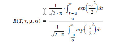
Observe that the limits for in the numerator correspond to time t=τ to infinity and in the denominator to time t=0 to infinity. The denominator therefore can be regarded as a normalising factor to take into account that negative values of do not exist so that the times to failure for systems subject to wear-out follow a truncated normal distribution.
Prior to hardware testing, values of estimated mean life (μ) and assumed standard deviation (σ) should be used in the above expression. Values of standard deviation generally lie between one-sixth and one-third of the mean life value, and so an average standard deviation should be assumed equal to one-quarter of the estimated mean life value.
Figure 3-4 shows, as an example, the failure-time density functions applicable to an item with a mean life (σ) of 300 hours, for standard deviation value (σ) equal to 50 hours (μ/6), 75 hours (μ/4) and 100 hours (μ/3).
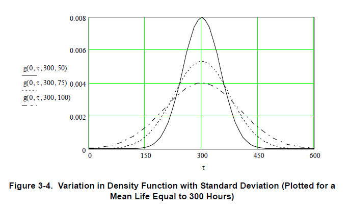
It can be seen that as the standard deviation increases, wear-out failures are more widely distributed about the mean life time. Hence, the larger the standard deviation, the earlier wear-out failures begin to affect reliability. The reliability associated with failure-time density function can be determined by integration, because:

Figure 3-5 shows a plot of this reliability function for each density function plotted in Figure 3-4. It should be noted that wear-out failures are negligible up to t=30 hours (i.e., one-tenth of the estimated mean life ). Providing the standard deviation applicable to the item's life is < μ/6, wear-out failures can be assumed negligible up to t=150 hours (i.e., one-half of the estimated mean life μ).
The predicted reliabilities of wear-out items, derived as shown in Figure 3-5, should be combined with the reliability values for constant failure rate items according to the relationships shown in the system reliability model.

Figure 3-6 shows, as another example, the failure-time density functions applicable to an item with a mean life (μ) of 100 hours, for standard deviation value (σ) equal to 50 hours (μ/6), 75 hours (μ/4) and 100 hours (μ/3).

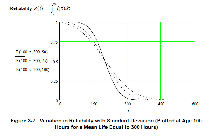
The predicted reliabilities of wear-out items, derived as shown in Figure 3-7, should be combined with the reliability values for constant failure rate items according to the relationships shown in the system reliability model.