Availability and State Probabilities
Assume that the system has only two states: state 1 is good, and state 2 is failed. Initially, the system is in a good state. The system reaches a failed state immediately after the single component fails. Repair of the component will start immediately after failure. Let λ and μ be the failure and repair rates of the single component. Figure 8-6 shows the state transition diagram for this system.

The information in the state transition diagram above can be represented in matrix form:

The matrix T is called a state transition rate matrix. The elements tij (row I and column j) represent the transition rate from state I to state j.
The matrix T is a square matrix of order n x n(where n is the total number of states), and all elements in the diagonal are zeros. In this example, n=2 |
Let PI(t) be the probability of state I at time t. Alternatively PI(t), is the probability that the system would be found in state I at time t. From the initial condition, it is known that the system is initially in state 1. Therefore, P1(0)=1 and P2(0)=0.
The initial state vector can also be represented in the matrix (vector) form:
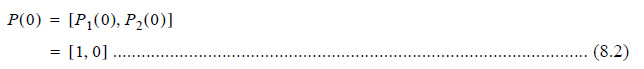
Where:
P(0)=The initial state vector, which is a row vector.
According to the definition, P1(t+Δt) is the probability of state I at time (t+Δt). Let Δt be very small, such that probability of occurrence of more than one event within this time interval (Δt) is negligible. Therefore, P1(t+Δt) can be expressed as the sum of the following two mutually exclusive events.
• E1–The system is in state 1 at time t and continues to remain in state 1 throughout the interval Δt.
• E2–The system is in state 2 at time t and it transitions to state 1 during the interval Δt.
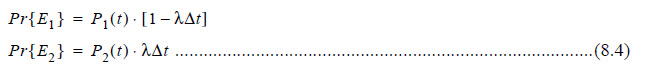
Therefore:

Where:
Pr{EI} = The probability of event EI.
According to the definition of the transition rates, if Δt is very small, the probability that the system transitions to state 2 from state 1 within Δt is λΔt. Using this same logic for the transition from state 2 to state 1 results in:
Therefore:

Similarly, P2(t+Δt) can be expressed as:

These equations for PI(t+Δt) are known as Chapman-Kolmogorov difference equations.
Rearranging equations (8.5) and (8.6) results in:

If Δt→0, then equation (8.7) can be represented in the form of differential equations:

Equation (8.8) can be represented in matrix form:

In a compact form, the equation is:

Where P`(t) and P(t)are the row vectors.
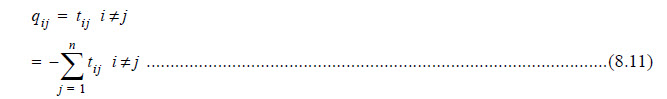
The matrix Q is known as an infinitesimal generator matrix of the Continuous Time Markov Chain (CTMC). It can be obtained directly from the transition matrix, T. Let qij and tij be elements of row I and j column of matrix Q and T respectively.
Then:
Equation (8.10) is known as a Kolmogorov (Forward) differential equation. The probability vector P(t) can be solved using the initial state probability vector P(0) and equation (8.10).
Similarly, the Kolmogorov (Backward) differential equation can be used to show the relationship between state probabilities. Equation (8.9) can be written as:

In a compact form, the equation is:

Where P`(t) and P(t) are the column vectors.
In some reference books, the symbol Q is used in the place of QT. Therefore, to avoid confusion, B is used to represent QT. The matrix B is also known as the coefficient matrix of the Markov differential equations.
In this chapter, the Kolmogorov backward differential equations are shown as in equation (8.13). There are various methods to solve this equation. This section presents the procedure to compute the probabilities analytically.
Taking a Laplace transform to equation (8.8) results in:

Where:

After solving equation (8.14), the following equations can be obtained:

PI(t) can be obtained after taking an inverse Laplace transform of PI(s).
Therefore:

Because the system is operational only in state 1, the availability of the system is A(t)=P1(t). Similarly, the reliability of the system, R(t), can be calculated as indicated in the next section.