Example: The Hilbert Transform
Use the hilbert function to create the Hilbert transform of a real signal such that the Discrete Fourier Transform of the analytic signal has magnitude zero at negative frequencies.
1. Use the sin and cos functions to define the input signal. Use the rnd function to add random noise.


2. Plot the input signal.
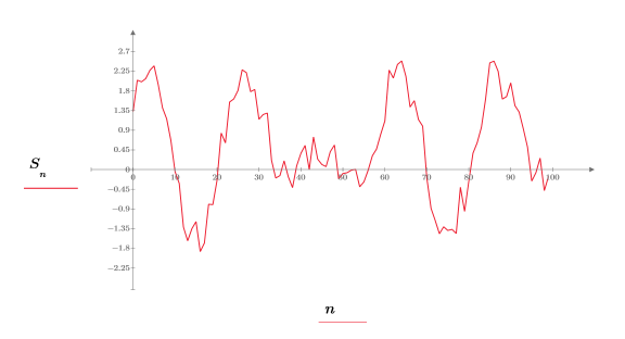
3. Use the hilbert function to compute the Hilbert transform of the input signal.

4. Plot the Hilbert transform signal.
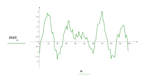
5. Build and plot the complex signal.

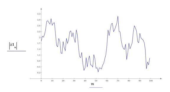
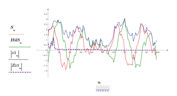
The next steps will show that the magnitude of the analytic signal is the complex envelope of the original signal.

7. Plot the absolute values of the spectrum.
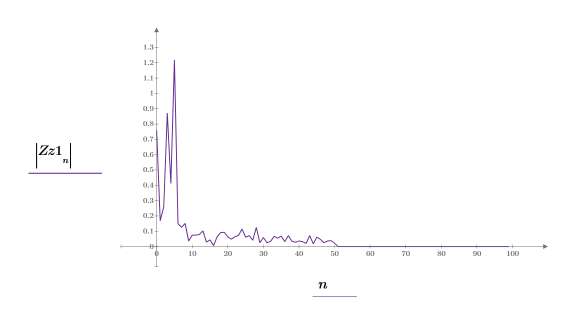
For vectors, the scaling factor between the dft function and the deprecated CFFT function is 1/N.
8. Plot all four signals on same graph.
The new signal that is created by Hilbert is related to the input signal in the transform domain in the following way:

where H is known as the Hilbert transformer, a filter with the frequency response:
 | for |  | |
 | for |  |
It is possible to build H through the filter design procedures and functions.
Ideal Hilbert Transformer
Rabiner and Gold (Theory and Application of Digital Signal Processing, Prentice-Hall, Inc.) give coefficients for an ideal Hilbert transformer. The examples below are based on the treatment in Section 14.4 of Signal Processing Algorithms, by Stearns and David (Prentice-Hall). The coefficients of the ideal filter are windowed and shifted to get a causal filter of odd length L.
1. Define the length and center.


2. Define the unwindowed coefficients h.
 | ||
 |  |  |
3. Use the hamming function to window the coefficients with a Hamming window, using the vectorize operator to multiply h and the window, element by element.


5. Plot the gain vs the frequency.
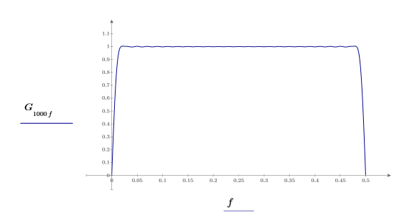
The frequency is normalized to sampling frequency of 1.
The filter has a delay of C, and we compute the phase shift of the filter relative to the delayed signal. The delay has this transfer function:
 | ||
 | ||
where: |  | |
 | ||
7. Plot the phase shift in degrees.
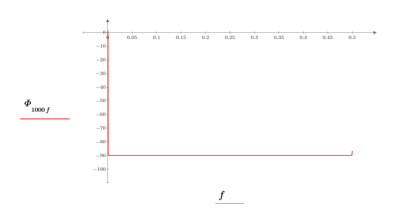
The shift is -90 degrees over almost the whole frequency range.
Testing the Filter
1. Define the signal parameters.


2. Use the exp function to create a new signal. The rnd function adds low frequency noise.

You may place the cursor on rnd and press F5 to recalculate and get a different random signal T.

3. Put the conjugates of these elements in the last 200 places of the signal to guarantee a real result when we invert it.

The new vector has 1001 elements where elements 1-200 contain the original vector T and elements 801-1000 contain the conjugates of T. In between elements are set to 0.
4. Find the Fourier transform of signal T.

Use the Re function to remove the small imaginary roundoff error. The noise is generated by building its transform T, using random phases and unit magnitudes for the first 200 elements after the first.
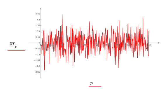
5. Plot the transformed signal.


7. Build a complex signal z2 using the first 800 elements of ZT and the last 800 elements of R.

Save the first 800 elements of the Fourier transform vector ZT into vector a2.

Save the last 800 elements of the response vector R into vector b2.

Define the complex signal z2.

8. Use the dft function to calculate the Discrete Fourier transform of signal z2.

For vectors, the scaling factor between the dft function and the deprecated CFFT function is 1/P.
9. Plot the absolute values of the Discrete Fourier transform of signal z2.
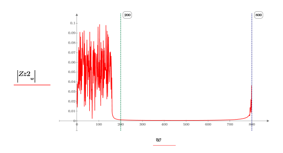
The original 200 points that were used to generate the signal in the transform domain are shown here. The upper half of the spectrum is essentially zero, so the Hilbert transformer filter has done its job.