Example: Signal Windowing
Use the following functions to perform signal windowing:
Ideal/Truncated Lowpass Impulse Response
1. Define the impulse response h of an ideal lowpass filter with normalized cutoff frequency 0.15.

2. Define the impulse response.

Since a realizable, finite-length filter must have a finite impulse response, this ideal response is truncated to some manageable number of terms.
3. To check the effect of direct truncation without windowing on the frequency response, define a length N filter that consists simply of the central N terms of the ideal response, shifted to make the filter causal.


As an exercise, set N to N2 and observe the effect of increasing the number of terms on the below examples.
4. Apply the impulse response function over the range of terms and plot the resulting function.


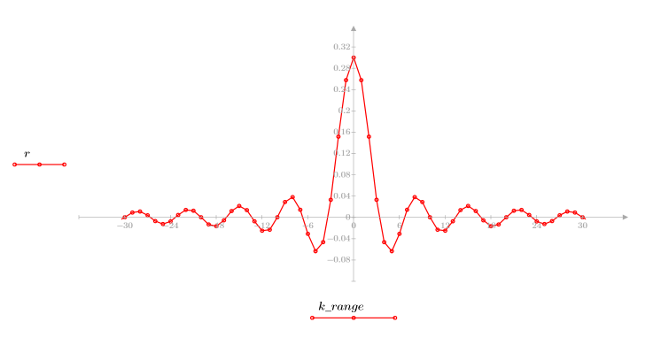
5. Calculate the frequency response for this truncated signal using the gain function, but first define the frequency range (multiples of sample frequency).


6. Collect the discrete magnitudes of the gain function into a new array.

7. Find the maximum magnitude of G and its corresponding frequency.


When number of terms equals N1=63, the maximum gain of 1.083 occurs at frequency freq=0.134.
When number of terms equals N2=127, the maximum gain of 1.092 occurs at frequency freq=0.142, thus moving closer to the band edge.
At frequency freq=0.2, the gain drops to almost zero. Compare the gain around this frequency in each of the following examples.
8. Plot the gain function over the defined range and show the frequency at which the magnitude has its maximum value.


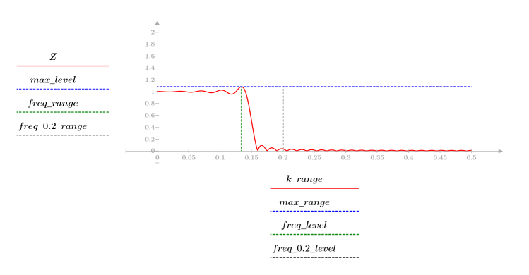
The overshoot at the edge of the passband is known as the Gibbs phenomenon. Increasing the filter order N from N1=63 to N2=127 above moves the overshoot closer to the band edge but doesn't decrease its amplitude.
The transition from 1 to 0 gets sharper with increased values of the filter order N.
One way to produce a more desirable frequency response is to window the ideal impulse response, so that the transition to 0 at the edges of the filter impulse response is smoother. Windows are multiplied term-by-term with a response vector r.
The Triangular Window
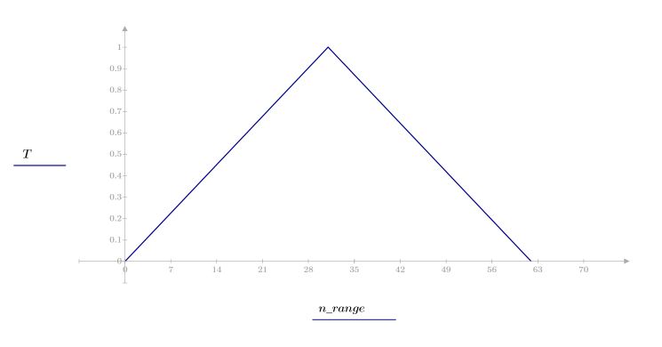
Function triangular returns the triangular or Bartlett window of width N.
The jth element of the resulting vector is given by:

for


for


1. Apply the function to filter order N and plot the resulting vector.

2. Calculate the windowed impulse response.

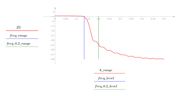
3. Use the gain function to calculate and plot the gain in dB of this filter, with coefficients vt, at frequency k/1000.


The Hanning Window
Function hanning returns the Hanning window of width N.
The kth element of the resulting vector is given by:

1. Apply the function to filter order N and plot the resulting vector.

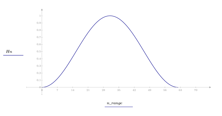
2. Calculate the windowed impulse response.

3. Use the gain function to calculate and plot the gain in dB of this filter, with coefficients vhn, at frequency k/1000.


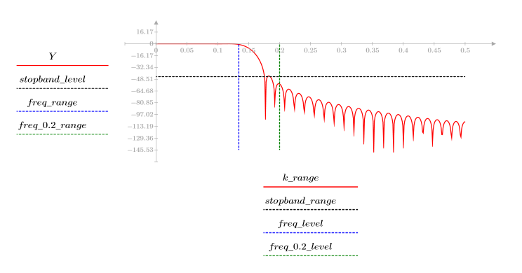
The stopband ripple is around -45 dB.
The Hamming Window
Function hamming returns the Hamming window of width N.
The kth element of the resulting vector is given by:

1. Apply the function to filter order N and plot the resulting vector.

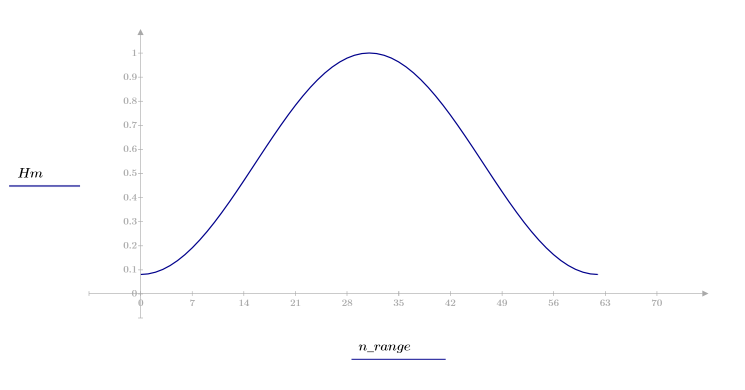
2. Calculate the windowed impulse response.

3. Use the gain function to calculate and plot the gain in dB of this filter, with coefficients vhm, at frequency k/1000.


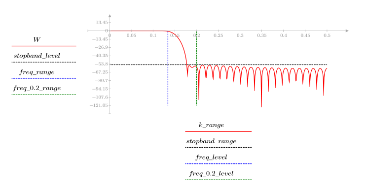
The stopband ripple is around -55 dB.
The Blackman Window
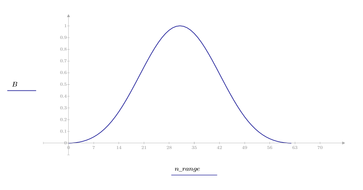
Function blackman returns the Blackman window of width N.
The kth element of the resulting vector is given by:

1. Apply the function to filter order N and plot the resulting vector

2. Calculate the windowed impulse response.

3. Use the gain function to calculate and plot the gain in dB of this filter, with coefficients vb, at frequency k/1000.


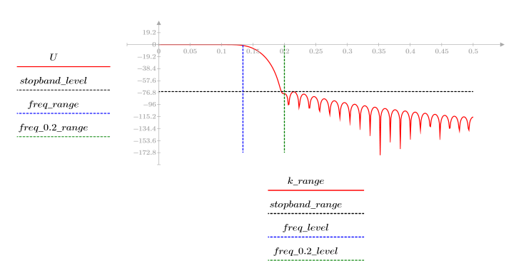
The stopband ripple is around -75 dB.
The Nuttall Window
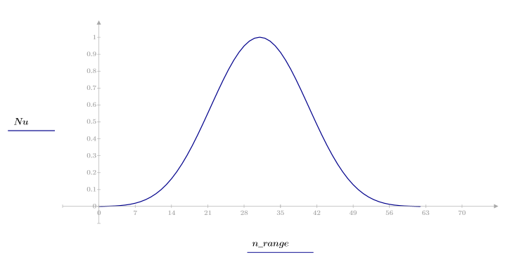
Function nuttall returns the Nuttall window of width N.
The kth element of the resulting vector is given by:

1. Apply the function to filter order N and plot the resulting vector.

2. Calculate the windowed impulse response.

3. Use the gain function to calculate and plot the gain in dB of this filter, with coefficients vnu, at frequency k/1000.


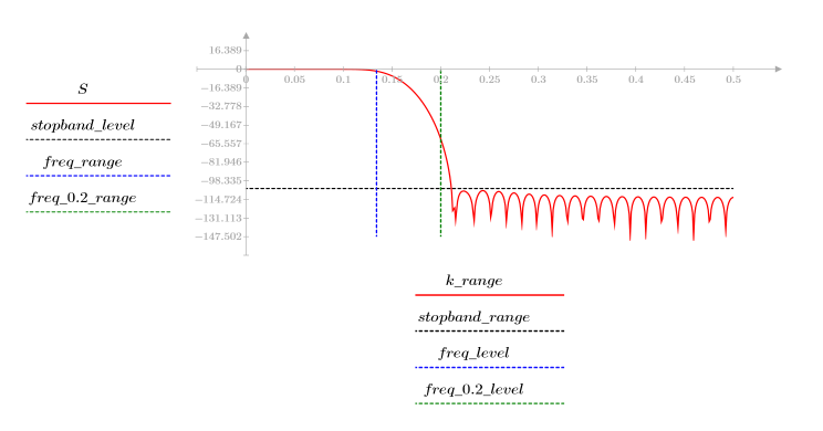
The stopband ripple is around -105 dB.
The Tapered Rectangular Window
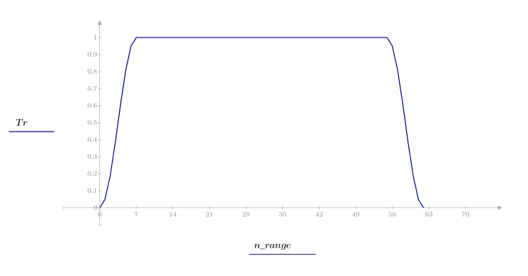
Function taprect returns the tapered rectangular window of width N.
This window is horizontal in the middle at a height of 1 with tapered ends formed from cosine curves. The right and left sides use the values:

where

and n runs from 0 to h.
1. Apply the function to filter order N and plot the resulting vector.

2. Calculate the windowed impulse response.

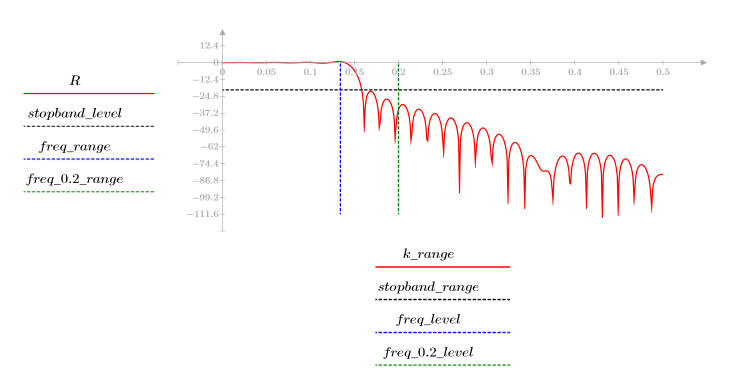
3. Use the gain function to calculate and plot the gain in dB of this filter, with coefficients vtr, at frequency k/1000.


The Gaussian Window
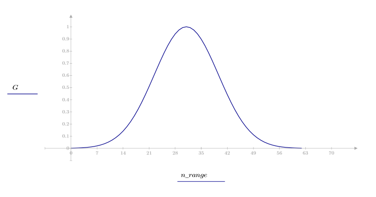
Function gaussian returns the Gaussian window of width N and parameter a. The number a is a real number proportional to the inverse of the Gaussian variance and must satisfy 2 < a < 20.
The kth element of the resulting vector is given by:

1. Apply the function to filter order N and plot the resulting vector.


2. Calculate the windowed impulse response.

3. Use the gain function to calculate and plot the gain in dB of this filter, with coefficients vg, at frequency k/1000.


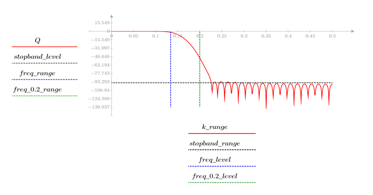
The stopband ripple is around -95 dB.
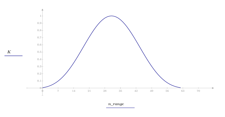
The Kaiser Window
Function kaiser returns the Kaiser window of width N and parameter b. The parameter b must satisfy 2≤b≤20.
The kth element of the resulting vector is given by:

1. Apply the function to filter order N and plot the resulting vector.


2. Calculate the windowed impulse response.

3. Use the gain function to calculate and plot the gain in dB of this filter, with coefficients vk, at frequency k/1000.


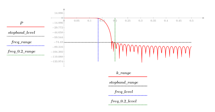
The stopband ripple is around -75 dB.
The Chebyshev Window
Function cheby returns the Chebyshev or equi-ripple window of width N and parameter b. The parameter b specifies the maximum side-lobe ripple in dB and must satisfy 1 < b; typically b is > 50. The length of this window must be odd. The Chebyshev window is computed by taking the inverse discrete Fourier transform of a Chebyshev polynomial evaluated at points around the unit circle. See Programs for Digital Signal Processing (IEEE Press) for more on this window.
1. Apply the function to filter order N and plot the resulting vector.


2. Calculate the windowed impulse response.

3. Use the gain function to calculate and plot the gain in dB of this filter, with coefficients vc, at frequency k/1000.


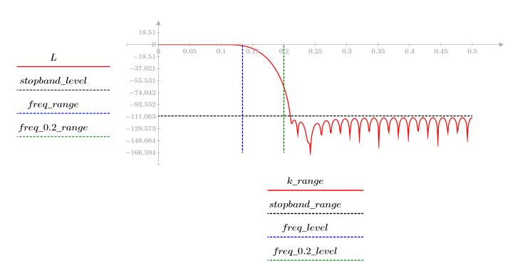
The stopband ripple is around -110 dB.
The Cosine Taper Window
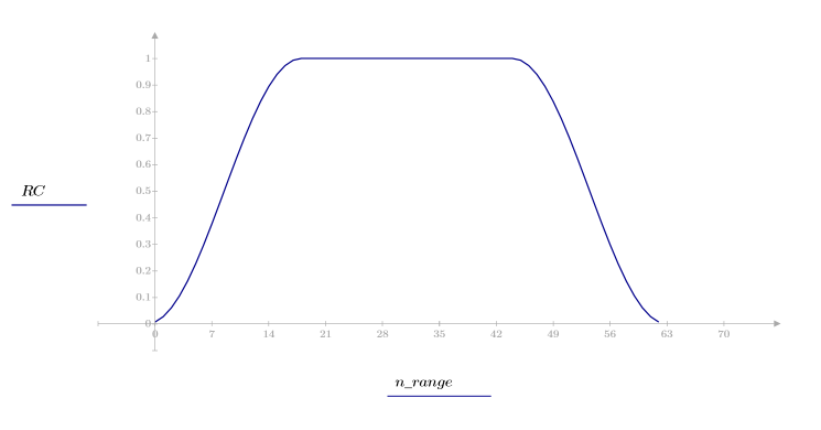
Function costaper is similar to the function taprect in that it returns a rectangular window with tapered tails that follow a cosine curve. However, you can use parameter a to specify the percentage of the window that should be created with a cosine curve. Parameter a should be between 0 and 1; a value of 0 returns a rectangular window, while a value of 1 returns a raised cosine curve.
For the tapered part of the window, the value of the kth element is given by:

where M is the number of window elements that fall in one of the tails, and is given by a-N:
1. Apply the function to filter order N and plot the resulting vector.


2. Calculate the windowed impulse response.

3. Use the gain function to calculate and plot the gain in dB of this filter, with coefficients vrc, at frequency k/1000.


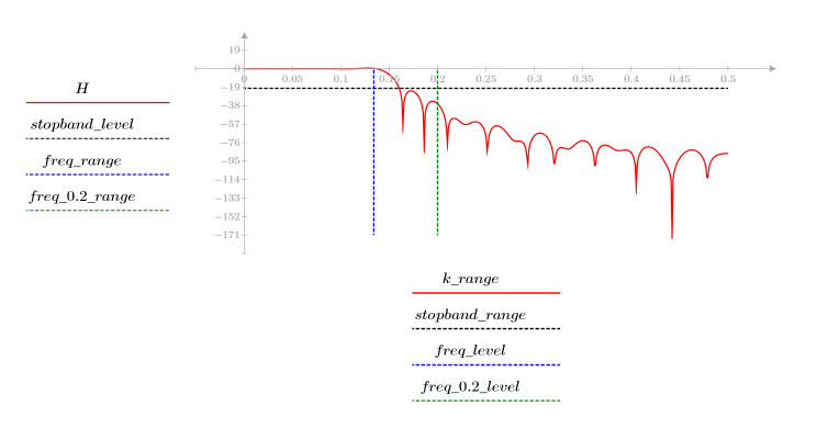
The stopband ripple is around -20 dB.
References
• S. Lawrence Marple, Jr., Digital Spectral Analysis with Applications, Prentice-Hall (1987).
• Lawrence R. Rabiner and Bernard Gold, Theory and Application of Digital Signal Processing, Prentice-Hall, Inc. (1975).
• T. W. Parks and C. S. Burrus, Digital Filter Design, Wiley-Interscience (1987).