Example: Principal Component Analysis 2
Use the Nipals and Nipals2 functions to analyze complex data such as near-infrared (NIR) spectra of pharmaceutical tablets with five different dosages of the active ingredients (the data is courtesy of Bruker Optics, Inc.). A model can be created to distinguish each dosage based on the spectrum, even though the actual dosages are not known. This model can be used for Quality Control purposes when producing further tablets.
1. Define the following data set:
|
|
This data set describes a double blind study in a clinical trial.
|

The first column is the wavenumber (1/wavelength), in cm-1. There are five sequential spectra of each dosage, constituting the remaining 25 columns.

3. Use the max and match functions to find the maximum value and the spectrum that contains it. Since the data values are very small, set TOL to an even smaller value.


The maximum value is in row 210 and column 17 of the Data matrix.
4. Plot the first two spectra of each dosage, which totals 10 data sets. The data set pairs are columns [1,2], [6,7], [11,12], [16,17], and [21,22] of the Data matrix.
◦ To get a reasonable scale for the horizontal axis, divide the wavenumbers by 1000. Similarly, since the spectra values are small, we multiply them by 1000.
◦ Use a horizontal marker to show the maximum spectra value.
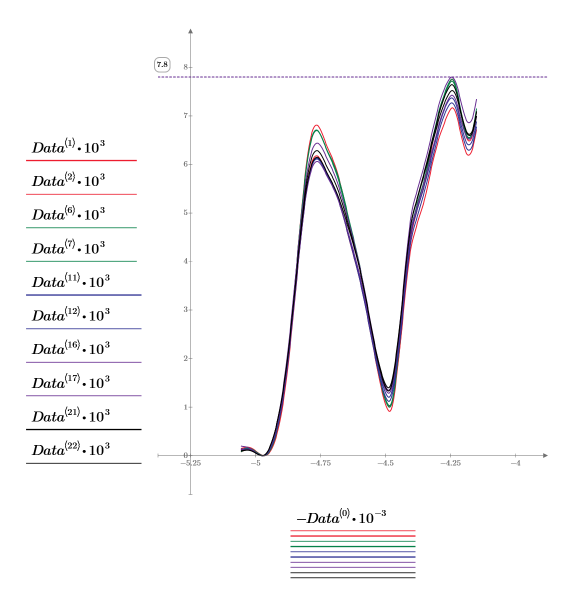
◦ By convention, wavenumbers are plotted in decreasing order. Data<0> is therefore negated to show the wavenumbers in the right order.
◦ No part of the spectrum can be used to easily distinguish one dosage from another: they all have the same basic form and close absorbance values.
◦ Most of the data are redundant. There are 236 points in each spectrum, which means 236 measured variables (absorbance for a particular wavelength of light), but the variation of these points is clearly interrelated.
5. Split the Data matrix into two data sets: the wavenumbers (column 0) and the spectra for each tablet (submatrix S). To match the common convention, transpose the spectra for each tablet so that each column corresponds to an independent variable.


6. Define the number of Principal Components, as well as the maximum number of iterations, before applying the Nipals function to the data. The Nipals function centers the data, subtracting the mean spectrum from each row.


7. Choose a spectrum to reconstruct.

8. Extract the scores and the loadings from the output of the Nipals function.


9. Use the mean function to calculate the mean spectrum.


10. Estimate of the original spectrum by multiplying the matrix of loading vectors with the matrix of scores, and then adding the mean spectrum.

11. Plot the original and the reconstructed spectrums. Scale the horizontal and vertical axes to get reasonable values.

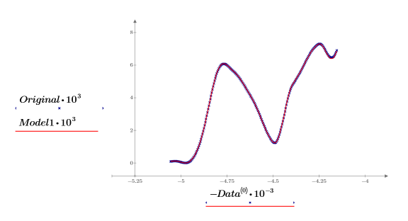
All the spectra are well represented using only two principal components for the principal component analysis.
12. Rearrange the scores into two matrices. Each column of the matrices represents the scores for one of the five tablet dosages.


13. Plot the scores of the first factor against the scores of the second factor. Each dosage is shown in a different color.
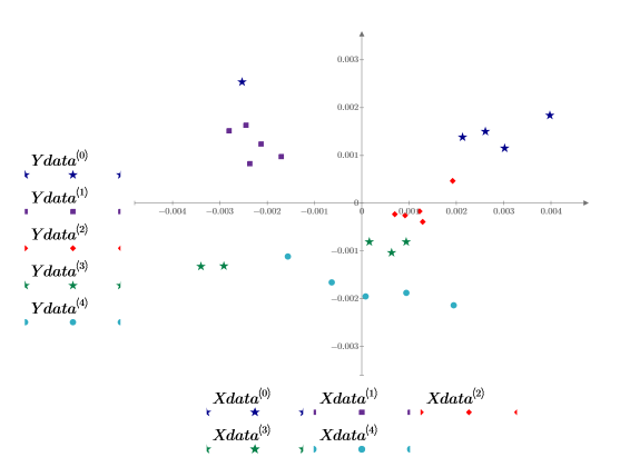
Some grouping of the data is evident, but it is still hard to distinguish one dosage from another. Adding a third score to the plot might help.
14. Use the Nipals2 function to add four principal components to the model created with two principal components.


The output matrix of NIPALS2 has the same form as that of NIPALS, but with additional columns and rows corresponding to the additional principal components. The number of scores and loadings has now increased to 6.
15. Extract the loadings and the scores from the NIPALS2 matrix to create a new model of the chosen spectrum.


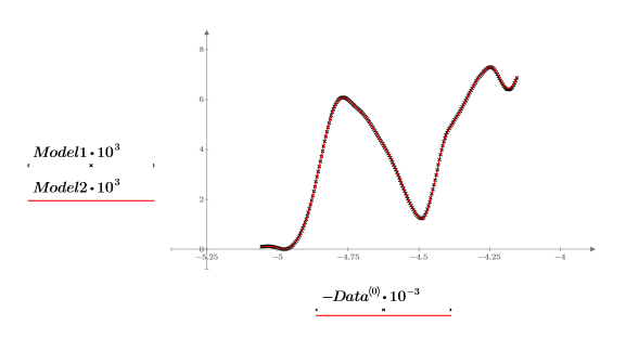
16. Plot and compare the two models for the chosen spectrum. Scale the horizontal and vertical axis to get reasonable values.
17. Extract the cumulative variance from NIPALS2.

18. Plot the cumulative variance against the number of principal components.


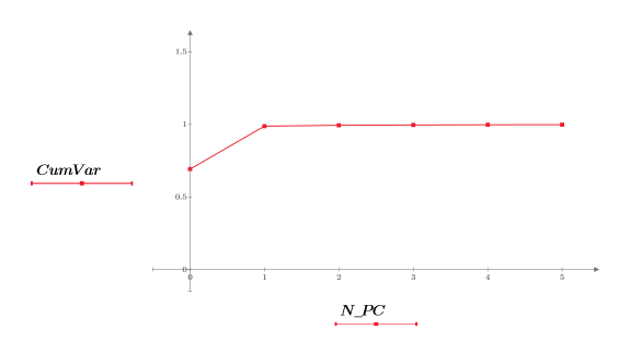
Although the first two principal components (PC) represent 99% of the variance, it is the third PC that is key to grouping the data by dosage. Principal component analysis compresses the data to the most dominant factors, but not the most relevant factors.