Example: Principal Component Analysis 1

Functions > Data Analysis > Principal Component Analysis > Example: Principal Component Analysis 1

Use the Nipals, loadings, scores, PCAeigenvals and PCAvariance functions to perform Principal Component Analysis (PCA).

The Nipals Function

1. Define a data set where each column stands for one variable.

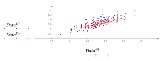
2. Plot the data set.

<region id="ID0EVHQU" top="364.80000000000007" left="38.400000000000006" height="214" width="575" xmlns="http://schemas.mathsoft.com/worksheet50">
  <plot background-type="white">
    <xyPlot>
      <title class="- topic/title " wwtype:type="Paragraph" xmlns:wwtype="urn:WebWorks-Type-Schema" />
      <legend />
      <traces>
        <trace resultRef="128">
          <traceStyle color="#FF00008B" symbol="x" line-weight="1" line-style="None">lines</traceStyle>
        </trace>
        <trace resultRef="129">
          <traceStyle color="#FFFF0000" symbol="x" line-weight="1" line-style="None">lines</traceStyle>
        </trace>
      </traces>
      <graph-size width="436.6" height="137.2" />
      <axes>
        <xAxis rank="1" legend-position="PlotBoundaryBottom" start="2.6" end="4.6">
          <axisLine position="ticknumberlock" positionticmark="0" legendWidth="100.183333333333" />
          <axisGrid>
            <gridFrequency>6</gridFrequency>
            <gridLabels display="true" />
            <gridLines />
            <tickMarks display="true" />
          </axisGrid>
          <axisLabel />
          <markers />
          <numberFormat>
            <general precision="3" show-trailing-zeros="false" radix="dec" zero-threshold="15" imaginary-value="i" exponential-threshold="3" />
          </numberFormat>
          <plotEquations>
            <plotEquation>
              <math resultRef="136">
                <apply xmlns="http://schemas.mathsoft.com/math50">
                  <matcol />
                  <id xml:space="preserve">Data</id>
                  <real>0</real>
                </apply>
              </math>
              <math resultRef="137">
                <placeholder xmlns="http://schemas.mathsoft.com/math50" />
              </math>
            </plotEquation>
          </plotEquations>
          <xyDomain scale-type="linear" auto-scale="true">
            <startValue resultRef="131">
              <real xmlns="http://schemas.mathsoft.com/math50">2.6</real>
            </startValue>
            <secondTickValue resultRef="133">
              <real xmlns="http://schemas.mathsoft.com/math50">3.0</real>
            </secondTickValue>
            <endValue resultRef="135">
              <real xmlns="http://schemas.mathsoft.com/math50">4.5</real>
            </endValue>
          </xyDomain>
        </xAxis>
        <yAxis rank="1" legend-position="PlotBoundaryLeft" start="2" end="5">
          <axisLine position="ticknumberlock" positionticmark="0" legendWidth="100.183333333333" />
          <axisGrid>
            <gridFrequency>7</gridFrequency>
            <gridLabels display="true" />
            <gridLines />
            <tickMarks display="true" />
          </axisGrid>
          <axisLabel />
          <markers />
          <numberFormat>
            <general precision="3" show-trailing-zeros="false" radix="dec" zero-threshold="15" imaginary-value="i" exponential-threshold="3" />
          </numberFormat>
          <plotEquations>
            <plotEquation>
              <math resultRef="144">
                <apply xmlns="http://schemas.mathsoft.com/math50">
                  <matcol />
                  <id xml:space="preserve">Data</id>
                  <real>1</real>
                </apply>
              </math>
              <math resultRef="145">
                <placeholder xmlns="http://schemas.mathsoft.com/math50" />
              </math>
            </plotEquation>
            <plotEquation>
              <math resultRef="146">
                <apply xmlns="http://schemas.mathsoft.com/math50">
                  <matcol />
                  <id xml:space="preserve">Data</id>
                  <real>2</real>
                </apply>
              </math>
              <math resultRef="147">
                <placeholder xmlns="http://schemas.mathsoft.com/math50" />
              </math>
            </plotEquation>
          </plotEquations>
          <xyDomain scale-type="linear" auto-scale="true">
            <startValue resultRef="139">
              <real xmlns="http://schemas.mathsoft.com/math50">2</real>
            </startValue>
            <secondTickValue resultRef="141">
              <real xmlns="http://schemas.mathsoft.com/math50">2.5</real>
            </secondTickValue>
            <endValue resultRef="143">
              <real xmlns="http://schemas.mathsoft.com/math50">5.0</real>
            </endValue>
          </xyDomain>
        </yAxis>
      </axes>
    </xyPlot>
  </plot>
</region>

In this graph, the x-y plane and the x-z plane are superimposed to expose the trend in the data. The data is in fact an elliptical cloud of points that almost lies on a plane. The three variables are linearly related, and the deviation from a perfect plane is due to noise.

3. Use the rows and cols functions to define the row and column indices.

4. Use the mean function to find the mean of the data and then subtract it from each variable in order to center the data.

<region id="ID0ETMQU" top="883.20000000000016" left="38.400000000000006" height="36.800000000000004" width="190.07" xmlns="http://schemas.mathsoft.com/worksheet50">
  <math resultRef="166">
    <define xmlns="http://schemas.mathsoft.com/math50">
      <apply>
        <indexer />
        <id labels="*" xml:space="preserve">C</id>
        <sequence>
          <id labels="*" xml:space="preserve">i</id>
          <id labels="*" xml:space="preserve">j</id>
        </sequence>
      </apply>
      <apply>
        <minus />
        <apply>
          <indexer />
          <id labels="VARIABLE" xml:space="preserve" label-is-contextual="true">Data</id>
          <sequence>
            <id xml:space="preserve">i</id>
            <id xml:space="preserve">j</id>
          </sequence>
        </apply>
        <apply>
          <indexer />
          <id labels="VARIABLE" xml:space="preserve" label-is-contextual="true">MeanData</id>
          <id xml:space="preserve">j</id>
        </apply>
      </apply>
    </define>
    <resultFormat>
      <matrix size="12,12" offset="0,0" show-indices="false" expand-nested-arrays="false" />
    </resultFormat>
  </math>
</region>

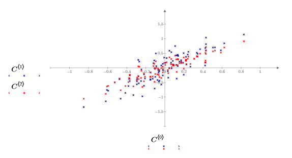
5. Plot the centered data.

<region id="ID0EDOQU" top="960.00000000000011" left="38.400000000000006" height="312" width="574" xmlns="http://schemas.mathsoft.com/worksheet50">
  <plot background-type="white" origin-positioning="true">
    <xyPlot>
      <title class="- topic/title " wwtype:type="Paragraph" xmlns:wwtype="urn:WebWorks-Type-Schema" />
      <legend />
      <traces>
        <trace resultRef="168">
          <traceStyle color="#FF00008B" symbol="x" line-weight="1" line-style="None">lines</traceStyle>
        </trace>
        <trace resultRef="169">
          <traceStyle color="#FFFF0000" symbol="x" line-weight="1" line-style="None">lines</traceStyle>
        </trace>
      </traces>
      <graph-size width="454.8" height="235.2" />
      <axes>
        <xAxis rank="1" legend-position="PlotBoundaryBottom" start="-1" end="1">
          <axisLine position="origin" positionticmark="3" legendWidth="77.7566666666667" />
          <axisGrid>
            <gridFrequency>11</gridFrequency>
            <gridLabels display="true" />
            <gridLines />
            <tickMarks display="true" />
          </axisGrid>
          <axisLabel />
          <markers />
          <numberFormat>
            <general precision="3" show-trailing-zeros="false" radix="dec" zero-threshold="15" imaginary-value="i" exponential-threshold="3" />
          </numberFormat>
          <plotEquations>
            <plotEquation>
              <math resultRef="174">
                <apply xmlns="http://schemas.mathsoft.com/math50">
                  <matcol />
                  <id xml:space="preserve">C</id>
                  <real>0</real>
                </apply>
              </math>
              <math resultRef="175">
                <placeholder xmlns="http://schemas.mathsoft.com/math50" />
              </math>
            </plotEquation>
          </plotEquations>
          <xyDomain scale-type="linear" auto-scale="true">
            <startValue resultRef="171">
              <real xmlns="http://schemas.mathsoft.com/math50">-1.</real>
            </startValue>
            <endValue resultRef="173">
              <real xmlns="http://schemas.mathsoft.com/math50">1.0</real>
            </endValue>
          </xyDomain>
        </xAxis>
        <yAxis rank="1" legend-position="PlotBoundaryLeft" start="-1.5" end="1.5">
          <axisLine position="origin" positionticmark="5" legendWidth="77.7566666666667" />
          <axisGrid>
            <gridFrequency>7</gridFrequency>
            <gridLabels display="true" />
            <gridLines />
            <tickMarks display="true" />
          </axisGrid>
          <axisLabel />
          <markers />
          <numberFormat>
            <general precision="3" show-trailing-zeros="false" radix="dec" zero-threshold="15" imaginary-value="i" exponential-threshold="3" />
          </numberFormat>
          <plotEquations>
            <plotEquation>
              <math resultRef="182">
                <apply xmlns="http://schemas.mathsoft.com/math50">
                  <matcol />
                  <id xml:space="preserve">C</id>
                  <real>1</real>
                </apply>
              </math>
              <math resultRef="183">
                <placeholder xmlns="http://schemas.mathsoft.com/math50" />
              </math>
            </plotEquation>
            <plotEquation>
              <math resultRef="184">
                <apply xmlns="http://schemas.mathsoft.com/math50">
                  <matcol />
                  <id xml:space="preserve">C</id>
                  <real>2</real>
                </apply>
              </math>
              <math resultRef="185">
                <placeholder xmlns="http://schemas.mathsoft.com/math50" />
              </math>
            </plotEquation>
          </plotEquations>
          <xyDomain scale-type="linear" auto-scale="true">
            <startValue resultRef="177">
              <real xmlns="http://schemas.mathsoft.com/math50">-1.5</real>
            </startValue>
            <secondTickValue resultRef="179">
              <real xmlns="http://schemas.mathsoft.com/math50">-1.0</real>
            </secondTickValue>
            <endValue resultRef="181">
              <real xmlns="http://schemas.mathsoft.com/math50">1.5</real>
            </endValue>
          </xyDomain>
        </yAxis>
      </axes>
    </xyPlot>
  </plot>
</region>

• The data is now centered about the origin. This is one of the steps that the Nipals function carries out automatically.

• In many applications of PCA, it is also desirable to scale the data so that the variables have equal weights, for example when different variables have different units. Scaling each variable (each column of Data) to unit variance is common, but not appropriate for this data, so no scaling is used here.

6. Use the Nipals function to create a new variable space. Use three principal components, which is the maximum possible since there were only three variables to start with.

<region id="ID0EDUQU" top="1612.8000000000002" left="38.400000000000006" height="25.6" width="499.89333333333337" xmlns="http://schemas.mathsoft.com/worksheet50">
  <math resultRef="203">
    <define xmlns="http://schemas.mathsoft.com/math50">
      <id labels="*" xml:space="preserve">NIPALS_Result</id>
      <apply>
        <id labels="FUNCTION" xml:space="preserve" label-is-contextual="true">Nipals</id>
        <sequence>
          <id labels="VARIABLE" xml:space="preserve" label-is-contextual="true">Data</id>
          <id labels="VARIABLE" xml:space="preserve" label-is-contextual="true">NumPC</id>
          <id labels="VARIABLE" xml:space="preserve" label-is-contextual="true">MaxIteration</id>
          <str xml:space="preserve">noscale</str>
          <id labels="VARIABLE" xml:space="preserve" label-is-contextual="true">Acc</id>
        </sequence>
      </apply>
    </define>
    <resultFormat>
      <matrix size="12,12" offset="0,0" show-indices="false" expand-nested-arrays="false" />
    </resultFormat>
  </math>
</region>

The output of the Nipals function is a nested matrix of 6 individual matrices. Use it to find the loadings, scores, eigenvals and eigenvecs of the data. If needed, use the Nipals2 function and the last two matrices to extract additional components.

Loadings and Scores

1. Call the loadings function to retrieve the data found in the second matrix of NIPALS_Result.

Each column of LOADINGS is a loading vector.

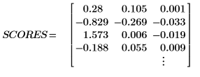
2. Call the scores function to retrieve the data found in the first matrix of NIPALS_Result.

The scores represent the proportions in which the loading vectors are added to recreate the original spectra. Think of them as intensities. Data = LOADINGS * SCOREST.

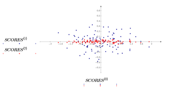
3. Plot the data stored in the SCORES matrix.

<region id="ID0ED5QU" top="2611.2000000000003" left="38.400000000000006" height="312" width="578" xmlns="http://schemas.mathsoft.com/worksheet50">
  <plot background-type="white" origin-positioning="true">
    <xyPlot>
      <title class="- topic/title " wwtype:type="Paragraph" xmlns:wwtype="urn:WebWorks-Type-Schema" />
      <legend />
      <traces>
        <trace resultRef="217">
          <traceStyle color="#FF00008B" symbol="x" line-weight="1" line-style="None">lines</traceStyle>
        </trace>
        <trace resultRef="218">
          <traceStyle color="#FFFF0000" symbol="x" line-weight="1" line-style="None">lines</traceStyle>
        </trace>
      </traces>
      <graph-size width="420.4" height="235.2" />
      <axes>
        <xAxis rank="1" legend-position="PlotBoundaryBottom" start="-2" end="2">
          <axisLine position="origin" positionticmark="5" legendWidth="130.073333333333" />
          <axisGrid>
            <gridFrequency>11</gridFrequency>
            <gridLabels display="true" />
            <gridLines />
            <tickMarks display="true" />
          </axisGrid>
          <axisLabel />
          <markers />
          <numberFormat>
            <general precision="3" show-trailing-zeros="false" radix="dec" zero-threshold="15" imaginary-value="i" exponential-threshold="3" />
          </numberFormat>
          <plotEquations>
            <plotEquation>
              <math resultRef="219">
                <apply xmlns="http://schemas.mathsoft.com/math50">
                  <matcol />
                  <id xml:space="preserve">SCORES</id>
                  <real>0</real>
                </apply>
              </math>
              <math resultRef="220">
                <placeholder xmlns="http://schemas.mathsoft.com/math50" />
              </math>
            </plotEquation>
          </plotEquations>
          <xyDomain scale-type="linear" auto-scale="true">
            <startValue>
              <placeholder xmlns="http://schemas.mathsoft.com/math50" />
            </startValue>
            <endValue>
              <placeholder xmlns="http://schemas.mathsoft.com/math50" />
            </endValue>
          </xyDomain>
        </xAxis>
        <yAxis rank="1" legend-position="PlotBoundaryLeft" start="-0.5" end="0.6">
          <axisLine position="origin" positionticmark="5" legendWidth="130.073333333333" />
          <axisGrid>
            <gridFrequency>12</gridFrequency>
            <gridLabels display="true" />
            <gridLines />
            <tickMarks display="true" />
          </axisGrid>
          <axisLabel />
          <markers />
          <numberFormat>
            <general precision="3" show-trailing-zeros="false" radix="dec" zero-threshold="15" imaginary-value="i" exponential-threshold="3" />
          </numberFormat>
          <plotEquations>
            <plotEquation>
              <math resultRef="227">
                <apply xmlns="http://schemas.mathsoft.com/math50">
                  <matcol />
                  <id xml:space="preserve">SCORES</id>
                  <real>1</real>
                </apply>
              </math>
              <math resultRef="228">
                <placeholder xmlns="http://schemas.mathsoft.com/math50" />
              </math>
            </plotEquation>
            <plotEquation>
              <math resultRef="229">
                <apply xmlns="http://schemas.mathsoft.com/math50">
                  <matcol />
                  <id xml:space="preserve">SCORES</id>
                  <real>2</real>
                </apply>
              </math>
              <math resultRef="230">
                <placeholder xmlns="http://schemas.mathsoft.com/math50" />
              </math>
            </plotEquation>
          </plotEquations>
          <xyDomain scale-type="linear" auto-scale="true">
            <startValue resultRef="222">
              <real xmlns="http://schemas.mathsoft.com/math50">-0.5</real>
            </startValue>
            <secondTickValue resultRef="224">
              <real xmlns="http://schemas.mathsoft.com/math50">-0.4</real>
            </secondTickValue>
            <endValue resultRef="226">
              <real xmlns="http://schemas.mathsoft.com/math50">0.5</real>
            </endValue>
          </xyDomain>
        </yAxis>
      </axes>
    </xyPlot>
  </plot>
</region>

The data has been rotated so that the maximum amount of variance can be explained by the first variable. This is represented on the graph by the long axis of the elliptical cloud, which is now parallel to the x-axis. The values for the third variable, parallel to the z-axis, are very small. For most purposes, this variable can be discarded. You have compressed the data.

PCA Variance and Eigenvalues

1. Use the PCAvariance function to return the cumulated variances of the three principal components.

The first two components make up 99.9% of the variance in the system.

2. Use the PCAeigenvals function to extract the eigenvalues of the principal components.