Example: Nonlinear Regression 2
Use the LeastSquaresFit function to perform nonlinear regression. The LeastSquaresFit solver gives the most flexibility for solving nonlinear regression problems. It allows you to enter constraint equations for any of the dependent parameters, lower and upper bounds on parameters, standard deviations on the x values, as well as a confidence limit for the calculation.
LeastSquaresFit
1. Define a data set.


This data is taken from an example discussed on the NIST website. The data was generated to 14-digits of accuracy using the following equation:

2. Define a fitting function.

The individual parameters above are elements of a vector β. You can also specify the input function with individual variable names, rather than elements of a vector:

3. Provide guess values.
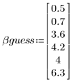
4. Define the confidence limit on the parameters.

5. Call the LeastSquaresFit function.

The solver uses sequential quadratic programming (SQP) to solve the resulting least-squares problem. By introducing additional variables, the original problem is transformed into a general equality constrained nonlinear programming problem, which is, in general, faster and more stable than some other methods.
6. View the output vector returned by the LeastSquaresFit function.
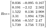
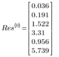
◦ The first column of output contains the values for the fitted parameters. The second column contains the left and the third column the right boundary for the confidence interval on the parameters.
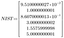
◦ The 95% confidence limits on the parameters cover a fairly wide range, showing that the fit is difficult and the individual parameters can vary widely. As a result, the values of the fitted parameters do differ from the correct values recorded on the NIST website:
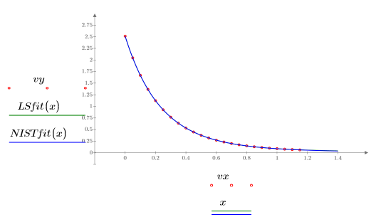
7. Plot the data, the Least Square fit and the NIST fit.


8. Compare the Least Square fit to the original data:


The fit is approaching convergence, but could benefit from an adjustment in the convergence tolerance. That can be done through one of the optional arguments of the LeastSquaresFit function.
Constraints, Standard Deviation, and Tolerance
There are several optional arguments to LeastSquaresFit:
• Standard deviation vector
• Lower and upper bounds matrix
• Accuracy
You can use any of the optional arguments alone, but if more than one argument is entered, the order of the arguments matters.
1. Perturb one of the data values, to simulate a mismeasurement.


2. Specify lower and upper bounds to constrain the fit values.
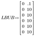
The bounds are set well outside the expected parameter values, because no particular bounds are known in this case.
3. Set a vector of standard deviations for each y value to mask the outlier.


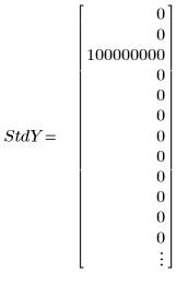
◦ The large value of 108 in the standard deviation effectively removes the mismeasurement from the calculation.
◦ When a vector of standard deviation is entered as an argument to the LeastSquaresFit function, the solver minimizes the following function

If the standard deviation is 0 for a point, then the original, undeviated function is used at that point, that is, StdYi is set to 1.
4. Set the accuracy to apply a more stringent convergence tolerance to the calculation (the default is 10-7).

5. Call the LeastSquaresFit function with and without the standard deviation.


◦ The unmasked calculation fails because the confidence limits are too large.
◦ The new parameters are closer to the NIST values:


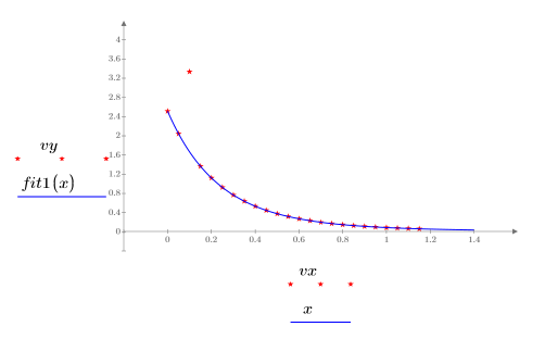
6. Plot the data with the outlier and the masked fit.


Reference
The data for this example is drawn from Lanczos, C., Applied Analysis, Prentice Hall, 1956, pages 272-280, as documented in the NIST Statistical Reference Dataset Archive.