Example: Noise Generators
Use the whiten, gaussn, and onefn functions for simulating white, Gaussian, and 1/f noises, respectively.
White Noise
The whiten function simulates the noise produced by N independent sources, each of which has random output following a uniform distribution between -0.5 and 0.5.
1. Use the whiten function to evaluate the white noise function for six independent noise sources.
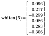
Repeated evaluation of the whiten function yields a different set of vector elements.
2. Consider a somewhat larger output vector.


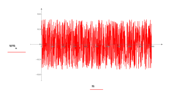
3. Plot the white noise function.
4. Use the mean and stdev functions to calculate the mean and standard deviation of the white noise vector.


5. Show the theoretical value of the mean, and then use the var function to calculate the standard deviation.
The plot shows that the wn signal has a theoretical mean of 0. | |
The standard deviation is the square root of the variance. |  |
6. Compare the calculated mean and standard deviation values with their theoretical values and verify that they do not deviate significantly from each other.
Gaussian Noise
The gaussn function simulates x number of independent noise sources, each following a Gaussian probability distribution of mean 0 and standard deviation 1.
1. Evaluate the gaussian noise function for six independent noise sources.
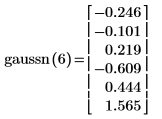
The elements of the vector can theoretically be any real value but will most likely lie between -3 and +3. You can verify this by pressing F5 to recalculate the function.
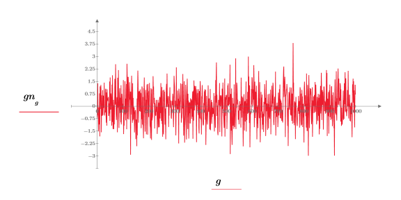
2. Plot a sample Gaussian sequence.


3. Prepare the Gaussian data for a bell-shaped histogram plot by grouping the values into 20, 0.05 wide, bins.


4. Define the vector that holds the edges of the bins, and then set the rightmost boundary.


5. Use the hist function to create the histogram, and then plot it as a bar graph.

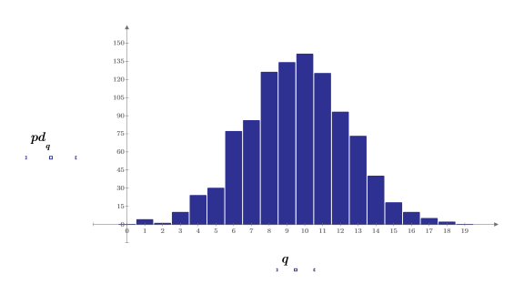
6. Compare the mean and standard deviation of the sample to the expected values of 0 and 1.


1/f Noise
The onefn function computes an approximation of 1/f noise using a routine based on an algorithm developed by Richard Voss (see Martin Gardner's column in Scientific American, April 1978).
1. Use the onefn function to generate a 1/f vector of 1000 points.


2. Adjust to mean 0.


3. Plot the vector data.
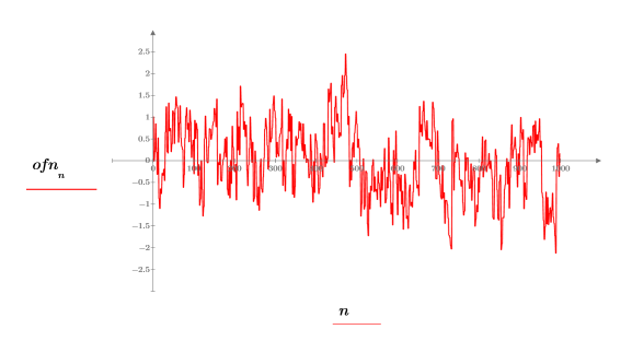
1/f noise is found in the signals of many natural and man-made phenomena, including music, brain signals, weather, stock market movements, and other hierarchically interacting systems. For example, if one were to digitize samples of a music of a variety of styles (rock, jazz, classical), one would find that their power spectra are very close in distribution to 1/f noise.
4. Use the lcorr function to compare the statistical structure of this noise with the white noise generated above by computing their autocorrelations.


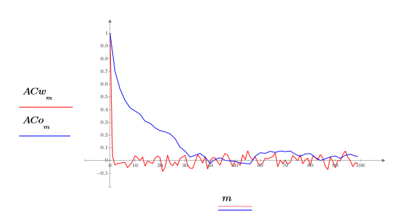
Unlike white noise, the noise generated by onefn is correlated, with the correlation decaying as the lag increases.
Comparison of Noise Signals Using Power Spectra
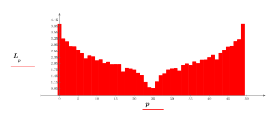
Another way of looking at differences between the white noise and 1/f noise is to compare their power spectra.
1. Assume 50 bins of frequency groups of 20.


2. Use the mag and dft functions to compute the magnitude squared of the frequency spectra for each signal.


3. Smooth the result by averaging over the frequency groups.


4. Plot the white noise spectrum.
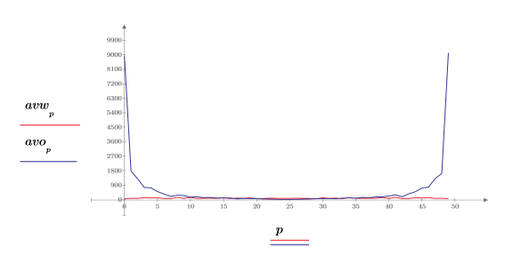
As expected, the white noise spectrum is essentially flat. The magnitude spectrum of the 1/f approximation falls off rapidly with increasing frequency.
5. Use the log function to calculate the more informative log of the magnitude.

Experiment
As an experiment, try constructing a 1/f power spectrum with random phases, and take the inverse transform to obtain the noise vector.
1. Define the width of the spectrum.


2. Use the exp function to construct the first half of the transform. A 1/f power spectrum corresponds to a 1/sqrt(f) magnitude spectrum.

3. Calculate the second half of the transform (For a real signal, the second half is conjugate-symmetric around the midpoint).

4. Set the mean of the noise to zero.

5. Use the idft function to get the inverse Fourier Transform (transform to the time domain).

6. Plot the real values of the inverse transform.
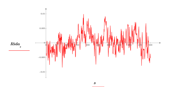
7. Use the lcorr function to calculate the autocorrelation curve.

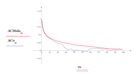
The behavior of the autocorrelation is similar to the output from onefn, with a correlation of 1.0 at 0 and varying degrees of correlation at other points.