Example: Identifying Influential Observations

Functions > Design of Experiments > Regression Analysis > Example: Identifying Influential Observations

Use function polyfitstat to test the observations used to create a multivariate polynomial regression.

1. Define a matrix that contains samples taken from 20 healthy individuals between 25 and 34 years old.

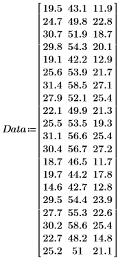
The columns of the matrix represent the triceps skinfold thickness, the thigh circumference, and the body fat, respectively, for each of the 20 individuals.

2. Use functions rows and cols to calculate the number of rows and columns.

3. Use the augment function to define matrix BM as the first two columns of the matrix. Use these measurements to predict the amount of fat in individuals.

4. Call polyfitstat to model the experiment by a first-order regression and to calculate the regression statistics.

5. Display the regression coefficients matrix found in row 7 of output matrix P.

6. Calculate the regression coefficients using matrix calculation.

The coefficients of regression fit the following equation:

7. Use the regression equation to calculate the predicted amount of body fat. Compare these values to the amount of body fat measured.

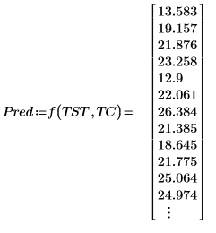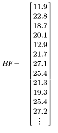8. Use the submatrix function to display model statistics found in the first rows of output matrix P.

<region id="ID0ESPCW" actualWidth="449.5" actualHeight="137.2" top="1996.8000000000002" left="38.400000000000006" xmlns="http://schemas.mathsoft.com/worksheet50">
  <math resultRef="125">
    <define xmlns="http://schemas.mathsoft.com/math50">
      <id labels="VARIABLE" xml:space="preserve">B</id>
      <eval>
        <apply>
          <id labels="*" xml:space="preserve">submatrix</id>
          <sequence>
            <id labels="VARIABLE" xml:space="preserve" label-is-contextual="true">P</id>
            <real>0</real>
            <real>6</real>
            <real>0</real>
            <real>1</real>
          </sequence>
        </apply>
        <unitOverride>
          <placeholder />
        </unitOverride>
      </eval>
    </define>
    <resultFormat>
      <general precision="3" show-trailing-zeros="false" radix="dec" zero-threshold="15" imaginary-value="i" exponential-threshold="3" />
      <matrix size="12,9" offset="0,0" show-indices="false" expand-nested-arrays="false" />
    </resultFormat>
  </math>
</region>

The first statistic is the standard deviation for the regression.

9. Display the model diagnostics found in the last nested matrix of output matrix P.

The observed and the predicted values correspond to the values displayed in step 7. The residuals are the difference between the observed and the predicted values:

10. Calculate the residuals, or the difference between the observed and the predicted values.

11. Use function diag to calculate the leverage values, or the diagonal values, of matrix H.

12. Calculate the studentized residuals.

The externally studentized residuals, or R-student, are calculated below. Constant p is the number of coefficients calculated for the regression and S2 is an estimate of s2 based on a data set where the ith observation is removed.

13. Use Cook's distance to measure the overall influence of a deleted point on a linear regression.

14. Calculate the difference between predicted values when all the observations are included in the fit and predicted values when the ith observation is omitted

<region id="ID0EJ3CW" actualWidth="182.92000000000002" actualHeight="87.502666332244885" top="3360.0000000000005" left="38.400000000000006" xmlns="http://schemas.mathsoft.com/worksheet50">
  <math resultRef="145">
    <define xmlns="http://schemas.mathsoft.com/math50">
      <apply>
        <indexer />
        <id labels="VARIABLE" xml:space="preserve">DFFITS</id>
        <id labels="VARIABLE" xml:space="preserve">i</id>
      </apply>
      <apply>
        <mult />
        <apply>
          <indexer />
          <id labels="VARIABLE" xml:space="preserve">
            <Span xmlns="http://schemas.microsoft.com/winfx/2006/xaml/presentation">R<Subscript xmlns="clr-namespace:Ptc.Wpf;assembly=Ptc.Core">St</Subscript></Span>
          </id>
          <id labels="VARIABLE" xml:space="preserve" label-is-contextual="true">i</id>
        </apply>
        <apply>
          <pow />
          <parens>
            <apply>
              <div />
              <apply>
                <indexer />
                <id labels="VARIABLE" xml:space="preserve" label-is-contextual="true">h</id>
                <id labels="VARIABLE" xml:space="preserve" label-is-contextual="true">i</id>
              </apply>
              <apply>
                <minus />
                <real>1</real>
                <apply>
                  <indexer />
                  <id labels="VARIABLE" xml:space="preserve" label-is-contextual="true">h</id>
                  <id labels="VARIABLE" xml:space="preserve" label-is-contextual="true">i</id>
                </apply>
              </apply>
            </apply>
          </parens>
          <apply>
            <div />
            <real>1</real>
            <real>2</real>
          </apply>
        </apply>
      </apply>
    </define>
    <resultFormat>
      <general precision="3" show-trailing-zeros="false" radix="dec" zero-threshold="15" imaginary-value="i" exponential-threshold="3" />
      <matrix size="12,9" offset="0,0" show-indices="false" expand-nested-arrays="false" />
    </resultFormat>
  </math>
</region>

15. Use functions augment and stack to display the above statistics.

<region id="ID0EP5CW" actualWidth="465.34000000000009" actualHeight="25.6" top="3494.4000000000005" left="38.400000000000006" xmlns="http://schemas.mathsoft.com/worksheet50">
  <math resultRef="147">
    <define xmlns="http://schemas.mathsoft.com/math50">
      <id labels="VARIABLE" xml:space="preserve">header</id>
      <matrix rows="1" cols="8">
        <str xml:space="preserve">Run</str>
        <str xml:space="preserve">Pred</str>
        <str xml:space="preserve">Res</str>
        <str xml:space="preserve">h</str>
        <str xml:space="preserve">St</str>
        <str xml:space="preserve">R.St</str>
        <str xml:space="preserve">C</str>
        <str xml:space="preserve">DFFITS</str>
      </matrix>
    </define>
    <resultFormat>
      <general precision="3" show-trailing-zeros="false" radix="dec" zero-threshold="15" imaginary-value="i" exponential-threshold="3" />
      <matrix size="12,12" offset="0,0" show-indices="false" expand-nested-arrays="false" />
    </resultFormat>
  </math>
</region>

<region id="ID0EL6CW" actualWidth="372.95000000000005" actualHeight="27.791200000000003" top="3571.2000000000007" left="38.400000000000006" xmlns="http://schemas.mathsoft.com/worksheet50">
  <math resultRef="151">
    <define xmlns="http://schemas.mathsoft.com/math50">
      <id labels="VARIABLE" xml:space="preserve">S1</id>
      <apply>
        <id labels="FUNCTION" xml:space="preserve" label-is-contextual="true">augment</id>
        <sequence>
          <id labels="VARIABLE" xml:space="preserve" label-is-contextual="true">run</id>
          <id labels="VARIABLE" xml:space="preserve" label-is-contextual="true">Pred</id>
          <id labels="VARIABLE" xml:space="preserve" label-is-contextual="true">Res</id>
          <id labels="VARIABLE" xml:space="preserve" label-is-contextual="true">h</id>
          <id labels="VARIABLE" xml:space="preserve" label-is-contextual="true">St</id>
          <id labels="VARIABLE" xml:space="preserve" label-is-contextual="true">
            <Span xmlns="http://schemas.microsoft.com/winfx/2006/xaml/presentation">R<Subscript xmlns="clr-namespace:Ptc.Wpf;assembly=Ptc.Core">St</Subscript></Span>
          </id>
          <id labels="VARIABLE" xml:space="preserve" label-is-contextual="true">C</id>
          <id labels="VARIABLE" xml:space="preserve" label-is-contextual="true">DFFITS</id>
        </sequence>
      </apply>
    </define>
    <resultFormat>
      <general precision="3" show-trailing-zeros="false" radix="dec" zero-threshold="15" imaginary-value="i" exponential-threshold="3" />
      <matrix size="12,12" offset="0,0" show-indices="false" expand-nested-arrays="false" />
    </resultFormat>
  </math>
</region>

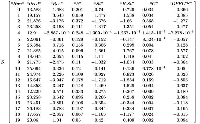
16. Use functions max and qt to determine the largest R-student value in the data set. Use the Bonferroni test to decide if the corresponding observation is an outlier.

The largest R-student value is smaller than the Bonferroni test which indicates that the corresponding observation is not an outlier.

17. Determine the maximum DFFITS value.

The value is larger than 1, but it is close enough to 1 that the corresponding observation is not necessarily influential.

18. Create an index influence plot by plotting the Cook's distances against the runs.

<region id="ID0EAHDW" actualWidth="577" actualHeight="312" top="4492.8000000000011" left="38.400000000000006" height="312" width="577" xmlns="http://schemas.mathsoft.com/worksheet50">
  <plot background-type="white" origin-positioning="true">
    <xyPlot>
      <title class="- topic/title " wwtype:type="Paragraph" xmlns:wwtype="urn:WebWorks-Type-Schema" />
      <legend />
      <traces>
        <trace resultRef="165">
          <traceStyle color="#FF00008B" symbol="x" line-weight="1" line-style="Solid">lines</traceStyle>
        </trace>
      </traces>
      <graph-size width="477" height="254.4" />
      <axes>
        <xAxis rank="1" legend-position="PlotBoundaryBottom" start="0" end="20">
          <axisLine position="origin" positionticmark="0" legendWidth="77.4766666666667" />
          <axisGrid>
            <gridFrequency>11</gridFrequency>
            <gridLabels display="true" />
            <gridLines />
            <tickMarks display="true" />
          </axisGrid>
          <axisLabel />
          <markers />
          <numberFormat>
            <general precision="3" show-trailing-zeros="false" radix="dec" zero-threshold="15" imaginary-value="i" exponential-threshold="3" />
          </numberFormat>
          <plotEquations>
            <plotEquation>
              <math resultRef="166">
                <id xml:space="preserve" xmlns="http://schemas.mathsoft.com/math50">run</id>
              </math>
              <math resultRef="167">
                <placeholder xmlns="http://schemas.mathsoft.com/math50" />
              </math>
            </plotEquation>
          </plotEquations>
          <xyDomain scale-type="linear" auto-scale="true">
            <startValue>
              <placeholder xmlns="http://schemas.mathsoft.com/math50" />
            </startValue>
            <endValue>
              <placeholder xmlns="http://schemas.mathsoft.com/math50" />
            </endValue>
          </xyDomain>
        </xAxis>
        <yAxis rank="1" legend-position="PlotBoundaryLeft" start="0" end="0.385">
          <axisLine position="origin" positionticmark="0" legendWidth="63.88" />
          <axisGrid>
            <gridFrequency>12</gridFrequency>
            <gridLabels display="true" />
            <gridLines />
            <tickMarks display="true" />
          </axisGrid>
          <axisLabel />
          <markers />
          <numberFormat>
            <general precision="3" show-trailing-zeros="false" radix="dec" zero-threshold="15" imaginary-value="i" exponential-threshold="3" />
          </numberFormat>
          <plotEquations>
            <plotEquation>
              <math resultRef="168">
                <id xml:space="preserve" xmlns="http://schemas.mathsoft.com/math50">C</id>
              </math>
              <math resultRef="169">
                <placeholder xmlns="http://schemas.mathsoft.com/math50" />
              </math>
            </plotEquation>
          </plotEquations>
          <xyDomain scale-type="linear" auto-scale="true">
            <startValue>
              <placeholder xmlns="http://schemas.mathsoft.com/math50" />
            </startValue>
            <endValue>
              <placeholder xmlns="http://schemas.mathsoft.com/math50" />
            </endValue>
          </xyDomain>
        </yAxis>
      </axes>
    </xyPlot>
  </plot>
</region>

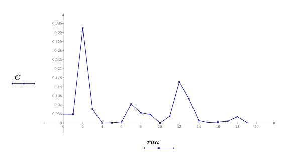
The observation for run2 is the most influential observation of the data set. The observation for run12 identified in step 10 is also influential but much less than that for run2.

Reference

Reference: Neter, J., Kutner, M.H., Nachtsheim, C.J., Wasserman, W., Applied Linear Statistical Models, 4th ed., McGraw-Hill/Irwin, Boston, 1996, pp. 375