Numerical Considerations
In homogeneous multiphase models, without considering velocity slips, no special treatment is required for solving the mixture momentum equations and formulation of face volume flux. This is because they are the same as those equations that govern the variable density single-phase flows. This topic focuses on the construction of the pressure-correction equation, and the treatment of the phase volume fraction equations, most notably, the interface resolving schemes in the VOF model.
Volume Continuity Equation
To satisfy the continuity constraint and ensure numerical stability, the pressure-correction equation is built based on total volume continuity instead of mass continuity. When you divide the q
th phase continuity /volume fraction
equation 2.57 by a phase reference density, ρ
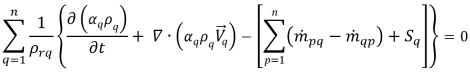
rq, and combine all the phases together, you get a total volume continuity equation which satisfies the law of mass conservation:
equation 2.135
where the phase reference density is usually set as the phase density, ρrq = ρq
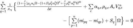
Introducing Ω as the volume of a computing cell, and integrating
equation 2.135 over the control volume, generates the discretized algebraic equations:
equation 2.136
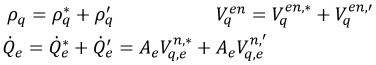
If you use the same approach as in the single phase pressure-based solver described in Numerics, and assume the following:
equation 2.137
equation 2.138
you can rearrange
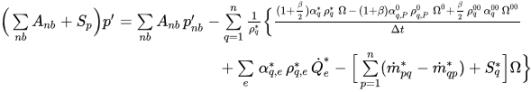
equation 2.136 as the following correction equation:
equation 2.139
Here * and ’ represent old values and corrections.
Δt | time step |
Ae | area at face e |
| volume flux |
Following the same approach as in the single-phase pressure-based solver, apply the SIMPLE type of algorithms (Simple, SimpleC and SimpleS) to connect the velocity and pressure corrections and to obtain the pressure correction equation for multiphase flows:
equation 2.140
where,
Anb | linking coefficient |
Sp | linearized term |
Phase Volume Fraction Equations
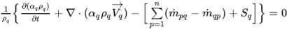
The transport of a phase volume fraction is governed by the phase mass conservation. Since the total volume conservation is applied in forming the pressure-correction equation, the actual equations solved for phase volume fractions are also in the form of volume conservation for numerical consistency:
equation 2.141
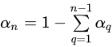
Usually, for an n phase system, only the (n–1) equations are solved, while the nth phase is obtained from the physical constraint:
equation 2.142
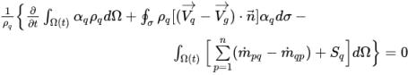
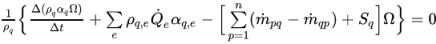
Following the discretizing approach, the integral form of
equation 2.141 is as follows:
equation 2.143
As given in the momentum, energy and total volume conservation equations, the spatial and temporal discretization schemes are crucial for numerical accuracy. For the volume fraction equations, in addition to the standard implicit time schemes, it is common practice to use the explicit time marching with high resolution advection schemes, so you can capture the interfaces in the VOF models more accurately. Both the implicit and explicit VOF formulations are described in detail in this section.
• VOF Implicit Formulation
With the VOF implicit formulation, the discretized phase volume fraction equation has the following general expression:
equation 2.144
In this equation, the phase volume fraction α
q at the current time step is a function of other quantities at the current time step. Therefore, as the momentum, energy and pressure correction equations, the discretized volume fraction
equation 2.144 is solved iteratively at each time step. In
Creo Flow Analysis, the implicit formulation adopted is summarized as follows:
◦ Advection Schemes—Volumetric flux

is computed based on the flow field at the current time step. The face value α
q,e is approximated in terms of the cell center values α
q,P,α
q,E and gradients (

,

) of neighboring cells P and E. As in the passive scalar equation, the advection schemes have the general form:
equation 2.145
Using different values for parameters γ, βP, and βE, and the schemes to calculate the volume fraction gradients, four advection schemes are developed for the volume fraction equations: First-Order Upwind, Second-Order Upwind, Center Difference, and High Resolution.
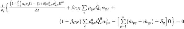
◦ Temporal Schemes—To describe the implicit temporal scheme, you can generalize
equation 2.144 in the following expression:
equation 2.146
The variables without a superscript are the values at the current time step. Variables with the superscript 0 or 00 indicate the values at the previous time steps.
Parameters β and βCN vary between 0 and 1and determining the time schemes. Specifically, three temporal schemes are adopted for the discretization of the phase volume fraction equations:
▪ Euler First-Order Upwind: β = 0, βCN = 1
▪ Three-Level Second-Order: β = 0, βCN = 1
▪ Crank-Nicolson Method: β = 0, βCN = 0.6 (default)
• VOF Explicit Formulation
When the explicit formulation is used for solving the VOF equations, the phase volume fractions at the current time step are directly calculated based on known quantities from the previous time step. Therefore, the VOF explicit formulation does not require an iterative solution for
equation 2.144 during each time step. However, since the rest of transport equations are solved implicitly, the time step for the volume fraction calculation is generally smaller than the time step for the other transport equations. A sub time step needs to be determined for the explicit VOF formulation, which is calculated automatically or which you can provide in
Creo Flow Analysis.
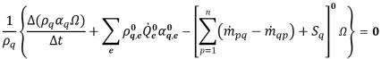
With the explicit formulation, the discretized phase volume fraction equation is formulated as:
equation 2.147
where both the advection and source terms are computed based on the known quantities from the previous time step. The volumetric flux

is computed in the same way as

in the implicit formulation. The face volume fraction

can also be estimated using one of the four advection schemes: First-Order Upwind, Second-Order Upwind, Center Difference, and High Resolution.
Creo Flow Analysis offers the following three algorithms for the explicit time marching schemes:
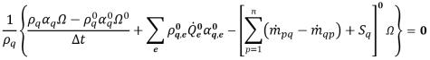
• Euler First Order Explicit—The volume fraction equation is discretized as follows:
equation 2.148
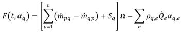
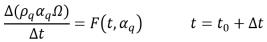
• Runge-Kutta Second-Order—Introducing the following function:
equation 2.149
equation 2.150
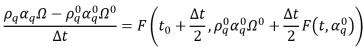
Then the second-order Runge-Kutta explicit scheme has the form:
equation 2.151
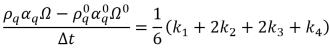
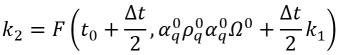
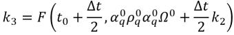
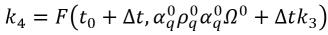
• Runge-Kutta Fourth-Order—For the phase q volume fraction equation, the fourth-order Runge-Kutta explicit scheme has the form:
equation 2.152
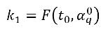
where
equation 2.153
equation 2.154
equation 2.155
equation 2.156
For the n phase system, typically only (n-1) phase volume fractions are solved, and the remaining one is obtained from the physical constraint,
equation 2.142. However, you can also solve all n phase volume fraction equations, and
equation 2.142 is satisfied by scaling each phase using the sum of the computed total volume fraction. This could be lesser or greater than 1 in an iterative process.