Flow Models
The
Flow module solves for conservation of mass and
momentum, using the transient Navier-Stokes Equations
H.Ding, F.C. Visser, Y.Jiang, and M. Furmanczyk, “Demonstration and Validation of a 3-D CFD Simulation Tool Predicting Pump Performance and Cavitation for Industrial Applications,” FEDSM2009-78256, 2009..
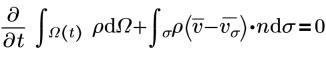
The integral form (conservative) of Reynold’s Averaged Navier-Stokes Equations (RANS) are as follows:
• Continuity
• Momentum
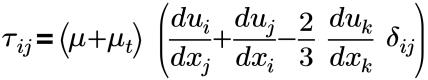
• Stress Tensor
where,
τij | effective shear stress (molecular+turbulent) |
f | body force |
n | surface normal |
ρ | static pressure(Pa) |
t | time |
v | fluid velocity |
vσ | mesh velocity |
Ω(t) | control volume as a function of time |
r | average local fluid density (kg/m3) |
σ | surface of control volume |
µ | dynamic viscosity (Poise or Pa-s) |
µt | turbulent dynamic viscosity |
δij | Kronecker delta(=1 for i=j, =0 for i≠j) |
Viscosity Models
• Constant Dynamic Viscosity—Specifies the fluid
viscosity in a selected volume. The unit of dynamic viscosity is Pa-s or N-s/m
2.
The value of the dynamic viscosity is specified in the box under the Constant Dynamic Viscosity selection.
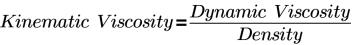
• Constant Kinematic Viscosity—Specifies the fluid
viscosity in a selected volume. The unit of kinematic viscosity is m
2/s. The value of the kinematic viscosity is specified in the box under the
Constant Kinematic Viscosity selection.
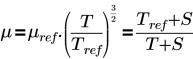
• Sutherland Law—Specifies the fluid
viscosity in a selected volume in terms of the dynamic viscosity (Pa-s). The equation and inputs are as follows:
where,
T | temperature (K) |
µref | viscosity at reference temperature (Pa-s) |
S | Sutherland Temperature (K) |
|  T is the fluid Temperature (K) required as an input if the energy module is not active. |
Sutherland Law is used to compute the viscosity of an ideal gas as a function of temperature.
Sutherland, W. (1893), "The viscosity of gases and molecular force," Philosophical Magazine, S. 5, 36, pp. 507-531 (1893). The following table shows Sutherland's constant and reference temperature for selected gases. Ref:
en.wikipedia.org/wiki/viscosity.
Gas | S (K) | Tref (K) | mref (Pa-s) |
air | 120 | 291.15 | 18.27 e-6 |
nitrogen | 111 | 300.55 | 17.81 e-6 |
oxygen | 127 | 292.25 | 20.81 e-6 |
carbon dioxide | 240 | 293.15 | 14.8 e-6 |
carbon monoxide | 118 | 288.15 | 17.2 e-6 |
hydrogen | 72 | 293.85 | 8.76 e-6 |
ammonia | 370 | 293.15 | 9.82 e-6 |
sulphur dioxide | 416 | 293.65 | 12.54 e-6 |
helium | 79.4 | 273 | 19 e-6 |
NonNewtonian Viscosity Models
The nonNewtonian viscosity models are:
• Herschel-Bulkley Model
• Bingham Models
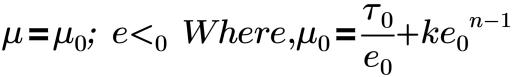
These models provide the appropriate viscosity for various types of fluids that exhibit nonNewtonian flow properties. The Herschel-Bulkley model and Bingham models relate the shear stress to the shear rate as follows:
where,
e0 | critical shear rate |
k | consistency index |
τ0 | yield stress of the fluid |
n | Power Law index. For Bingham model, n=1 |
| The shear rate of 0 is the same as the gamma dot in the plot above. |
Resistance Model
Resistance Model is a
Flow module option that you can use to set a resistance in a selected volume. The
Resistance Model contains the following two models:
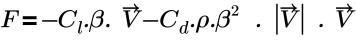
• Pressure Loss: based on the following equation:
where,
Cl | linear drag coefficient (Pa-s/m2) |
Cd | quadratic drag coefficient (1/m) |
β | porosity |
ρ | density |
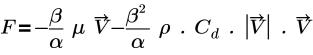
• Darcy's Law: model based on the following equation:
where,
β | porosity |
α | permeability |
µ | dynamic viscosity |
V | velocity |
Cd | quadratic drag coefficient (1/m) |
The velocity used in the resistance equation is the local velocity. F in the equation is measured in the unit N/m3, such as force/volume, or pressure gradient (Dp/Dx), or rg. The pressure drop across the interface is computed by multiplying F by a finite thickness. The porosity is set in the Common module.