Turbulent Flow in Diffuser: Exercise 7—Analyzing Results
This exercise describes how the results are analyzed during and after the simulation. To hide CAD surfaces (not the fluid domain), switch between  CAD Bodies and
  Flow Analysis Bodies in the Show group. Clear any variable display by selecting No Selection in the Legend drop-down. Click
  XYPlot Panel to view the XY Plot.
CAD Bodies and Flow Analysis Bodies in the Show group. Clear any variable display by selecting No Selection in the Legend drop-down. Click XYPlot Panel to view the XY Plot.1. To show/hide selected geometric entities, click  Show in View Panel. Show in View Panel.2. To change the color scheme, click on  More in the Legend and select between Blue Red and Blue Purple. More in the Legend and select between Blue Red and Blue Purple. |
Viewing the Pressure Contours on a Section
 | Pressure Pa 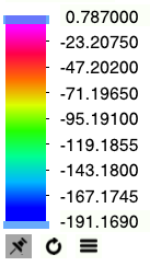 |

1. In the Post-processing group, click  Section View and create a section. Section 02 appears under Derived Surfaces.
Section View and create a section. Section 02 appears under Derived Surfaces.2. Select Section 02.
3. In the Properties panel, Model tab, set values for the options as listed below:
◦ Type — Plane Y
◦ Position — 0
4. In the Properties panel, View tab, for Surface, set values for the options as listed below:
◦ Grid—No
◦ Outline—Yes
◦ Variable — Pressure [Pa] : Flow
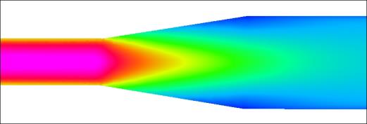
Viewing the Velocity Magnitude on a Section
 | Velocity Magnitude m/s 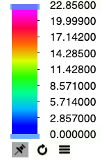 |
1. In the Post-processing group, click Section View and create a section. Section 03 appears under Derived Surfaces.
Section View and create a section. Section 03 appears under Derived Surfaces.2. Select Section 03.
3. In the Properties panel, Model tab, set values for the options as listed below:
◦ Type — Plane Y
◦ Position — 0
4. In the Properties panel, View tab, for Surface, set values for the options as listed below:
◦ Grid—No
◦ Outline—Yes
◦ Variable — Velocity Magnitude [m/s] : Flow
Plotting the Temperature at the Monitoring Point
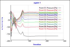
1. In the Flow Analysis Tree, under Results, click Monitoring Points..
2. Select Point01 to Point10.
3. Click  XYPlot. A new entity xyplot1 appears in the Flow Analysis Tree under >
XYPlot. A new entity xyplot1 appears in the Flow Analysis Tree under > 4. Click xyplot1.
5. In the Properties panel, View tab, for Surface, set Variable to Pressure [Pa] : Flow.
Plotting the Temperature at the Monitoring Point
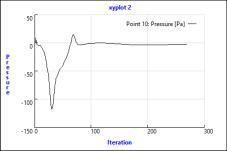
1. In the Flow Analysis Tree, under Results, click Monitoring Points..
2. Select Point10.
3. Click XYPlot. A new entity xyplot2 appears in the Flow Analysis Tree under >
XYPlot. A new entity xyplot2 appears in the Flow Analysis Tree under > 4. The monitoring point Point10 is added to xyplot2.
Validation
The coefficient of pressure at diffuser wall is calculated as follows:

where,
P | Pressure at the diffuser walls (Pa): From monitoring points |
ρ | Density (kg/m3): 1.15758 |
Pdiffuser | Pressure at the diffuser outlet (Pa): -2.6066 |
u | Inlet velocity m/s: 18.06 |
The monitoring points in the simulation are used to measure the pressure close to the diffuser wall:
Points | X | X/D | Static Pressure (Pa) | Pressure at Diffuser Outlet (Pa) | Coefficient of Pressure Cp |
|---|---|---|---|---|---|
Point01 | 3.500 | 0.000 | -170.453 | -2.293 | -0.891 |
Point02 | 3.575 | 0.738 | -106.429 | -2.293 | -0.552 |
Point03 | 3.650 | 1.476 | -72.543 | -2.293 | -0.372 |
Point04 | 3.725 | 2.215 | -51.002 | -2.293 | -0.258 |
Point05 | 3.800 | 2.953 | -36.504 | -2.293 | -0.181 |
Point06 | 3.875 | 3.691 | -26.172 | -2.293 | -0.126 |
Point07 | 3.950 | 4.429 | -18.522 | -2.293 | -0.086 |
Point08 | 4.025 | 5.167 | -12.885 | -2.293 | -0.056 |
Point09 | 4.100 | 5.906 | -8.056 | -2.293 | -0.031 |
Point10 | 4.218 | 7.067 | -2.293 | -2.293 | 0.000 |
where,
X/D= (X-3.5)/D and D (m) = 0.1016
The comparison of the coefficient of pressure from experiments and Creo Flow Analysis are as follows:
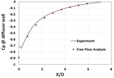
Reference: Azad, R. S., & Kassab, S. Z. (1989). Turbulent flow in a conical diffuser: Overview and implications. Physics of Fluids A: Fluid Dynamics, 1(3), 564–573.
Parent topic