Natural Convection: Exercise 8—Analyzing Results
This exercise describes how the results are analyzed during and after the simulation. To hide CAD surfaces (not the fluid domain), switch between  CAD Bodies and
  Flow Analysis Bodies.
CAD Bodies and Flow Analysis Bodies.Viewing the Temperature Contours on a Boundary
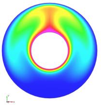 | Temperature: [K] : Heat 373  327.0 |
1. Under Domains, select CONCENTRIC_ANNULUS.
2. In the Properties panel, View tab, for Surface, set values for the options as listed below:
◦ Surface—Yes
◦ Grid—No
◦ Outline—No
◦ Variable—Temperature: [K] : Heat
◦ Min—327
◦ Max—373
Plotting the Temperature at the Monitoring Point
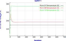
1. In the Flow Analysis Tree, under Results, click Monitoring Points..
2. Select Point01, Point08, Point10.
3. Click  XYPlot. A new entity xyplot1 appears in the Flow Analysis Tree under >
XYPlot. A new entity xyplot1 appears in the Flow Analysis Tree under > 4. Click xyplot1.
5. In the Properties panel, View tab, for Surface, set Variable to Temperature: [K]: Heat.
Viewing the Streamlines at the Domain
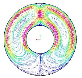 | Velocity Magnitude: [m/s] : Flow 0.074 0 |
1. In the Post-processing group, click  Stream Lines. Under
  Results > Streamlines, Streamline 01 is selected.
Stream Lines. Under Results > Streamlines, Streamline 01 is selected.2. In the Properties panel, Model tab, select the following values for the options listed:
◦ Line Thickness—0.0002
◦ Animation Time Size—0.05
3. In the Properties panel, View tab, under Surface, select the following values for the options listed:
◦ Variable—Velocity Magnitude: [m/s] : Flow
◦ Min—0.0
◦ Max—0.74
4. In the Flow Analysis Tree, under General Boundaries select inner_surface, bottom_surface, and top_surface.
5. In the Properties Panel, Model tab, for Streamline, set Release Particle to Yes and Number of Particles to 100.
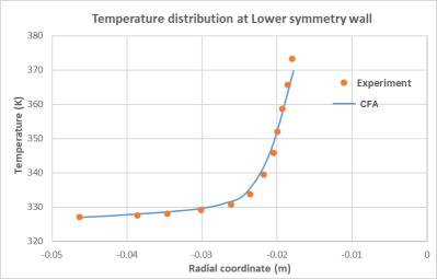
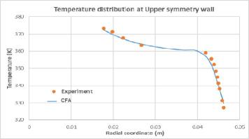
Validation
The temperature prediction along the radial direction on both the upper and lower symmetry walls are compared with experimental data from Kuehn & Goldstein.