Post-processing
The following options are available for analyzing the results in Creo Flow Analysis.
Contours
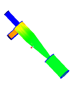 |
Pressure: [Pa] : Flow
101350.000000  101325.000000 |
To view volumes and boundaries follow the steps below:
1. In the Flow Analysis Tree, select a boundary.
2. In the Properties panel click the View tab.
3. Under Surface, specify the following values:
◦ Surface—Yes
◦ Variable—select the variable to display the contours
Section View
Sections, also referred to as cross-sections, are derived planar surfaces that slice through the domain or volumes at an orientation and location that you specify. Use sections to reveal features or display a Variable.
Create a section by following the steps below:
1. Click >  Flow Analysis. The Flow Analysis tab appears.
Flow Analysis. The Flow Analysis tab appears.2. Click  New Project.
New Project.3. In the Post-processing group, click  Section View. In the Flow Analysis Tree, under Derived Surfaces a new entity Section 01 is created.
Section View. In the Flow Analysis Tree, under Derived Surfaces a new entity Section 01 is created.4. Select Section 01.
5. In the Properties panel, click the Model tab.
6. Under Surface, specify the following values:
◦ Type—Plane X, Plane Y, Plane Z
◦ Position—drag the slider to adjust the position of the Section
Display Grid on a Section
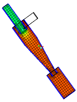 | Pressure: [Pa] : Flow 101343.937500  101313.132813 |
1. In the Flow Analysis Tree, under Derived Surfaces, select Section 01.
2. Specify the following values:
a. Surface—Yes
b. Grid—Yes
Contours for variables on a section
1. In the Flow Analysis Tree, under Derived Surfaces, select Section 01.
2. Under Surface, specify Variable—Density: [kg/m3] : Common or Cell Volume: [m3] : Common.
Monitoring Points
A point is a specified X, Y, Z coordinate within a model, used to record variables or property data at that location. The position of a point is associated with a given mesh cell based on its location at the start of a simulation. If the mesh moves, the point will move with the cell. When a point moves with the mesh, its new position is not graphically updated.
To create a monitoring point, follow the steps listed below:
1. Click Flow Analysis > .
Flow Analysis > .2. Click  Monitor Points. In the Flow Analysis Tree, a new entity Point 01 appears under Monitor Points.
Monitor Points. In the Flow Analysis Tree, a new entity Point 01 appears under Monitor Points.You can set the position of a point from the Properties panel.
Streamlines
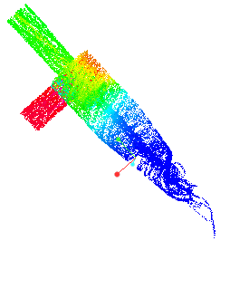 | Velocity Magnitude : [m/s] : Flow 5.969755  0.000000 |
Use streamlines to track the path of flow. Streamlines show the direction in which a fluid element travels at any point in time. The appearance of a streamline depends on the following:
• Line Thickness—Controls the thickness of streamlines. It is specified in terms of absolute value (m).
• Animation Time Size—When set to a nonzero positive real number, together with an assignment for streamline display variable, each streamline is divided into multiple sections. Each section keeps moving along the flow direction with a speed proportional to the local flow speed. The length of a streamline section equals the local velocity times the animation time size.
• Maximum Integral Steps—Limits how far the streamline algorithm tracks a streamline. This prevents the streamline module from using excessive computation time trying to track the streamline that is looping or near stagnant. A smaller value reduces the number of calculations, but may end a streamline earlier than desired.
To create a streamline, follow the steps listed below:
1. In the Flow Analysis Tree, select a domain.
2. Click  Physics Module. The Physical Model Selection dialog box opens.
Physics Module. The Physical Model Selection dialog box opens.3. Under Available Modules, double-click Streamline and click Add.
4. Click Close to close the Physical Model Selection dialog box. A new entity Streamline appears in the Flow Analysis Tree.
To enable a streamline, follow the steps listed below:
1. Select a general boundary from where the streamline should begin.
2. In the Properties panel, Model tab set Release Particle—Yes.
Isosurface
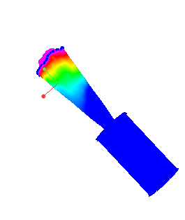 | Velocity Magnitude: [m/s] : Flow 1.000000  0.000000 |
Isosurfaces are surfaces that envelope regions less-than (Below Value), equal-to (Single Value), or greater than (Above Value), a specified scalar value of a selected Variable, derived variable, or Property. Isosurfaces can also envelope the region between two scalars using a Value Range.
To create an isosurface, follow the steps listed below:
1. Click Flow Analysis >  Isosurface.
Flow Analysis > Isosurface.2. In the Flow Analysis Tree, a new entity Isosurface 01 appears under Derived Surfaces.
The shape of an isosurface depends on theIsosurface Variable,Type, and Value set in the Properties panel.
XY Plots
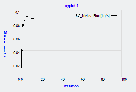
The quantitative results of the simulation are shown using the XY- Plots. Review the results on the boundaries or the volumes or on monitoring points, such as for mass flux, temperature, and so on.
To create an XY-plot, follow the steps listed below:
1. In the Flow Analysis tree, under Results, select a boundary.
2. In the Post-processing group, click  XYPlot. A new entity xyplot1 appears under Results in the Flow Analysis Tree.
XYPlot. A new entity xyplot1 appears under Results in the Flow Analysis Tree.3. Select this entity.
4. In the Properties panel under Variable, select the variable to be plotted.
Follow the steps below to select the variables to use as output in the plots:
1. Under General Boundaries select a boundary or under Domains select a volume.
2. In the Properties panel for each module set Output to User Select.
3. Set the required variables such as Pressure Force to Yes.
For details about output variables see Flow Output Variables, Turbulence Output Variables, Heat Output Variables.