Functions
The following functions in the Expression Editor enable mathematical and logical manipulation of vectors and scalars:
• Operators
◦ Common to Vectors and Scalars, such as addition and subtraction
◦ Scalars only, such as square roots and logs
◦ Vectors only, such as dot and cross products
• Logicals
• Trigonometric and Hyperbolic
• Other functions
• Tables
Operators
The operators enable mathematical manipulation of both vectors and scalars. In the following table a, b, c are scalars, and U, V, W are vectors.
|
Expression Operators
|
Function
|
Example
|
|---|---|---|
|
Operators: Scalars and/or Vectors
|
||
|
Addition
|
a = b+c or V = U+W
|
|
|
Subtraction
|
a = b-c or V = U-W
|
|
|
*
|
Multiplication of two Scalars or a Scalar and a Vector
|
a = b*c or V = a*U (but not V = U * W)
|
|
Operator: Scalars Only
|
||
|
/
|
Division
|
a = b/c
|
|
exp(scalar)
|
Base e exponential function
|
a= exp(b) raises e to the power of b: a= eb
|
|
ln(scalar)
|
The natural logarithm function for e
|
a= ln(b) returns the natural log of b
|
|
sqrt(scalar)
|
square root function
|
a = sqrt(b)
|
|
^
|
exponential function
|
a= b^c raises b to the power of c: a= bc
|
|
Operator: Vectors Only
|
||
|
&
|
vector dot product
|
a = V&U (a = |V| |U| cos (angle))
|
|
^
|
vector cross product
|
V=U^W (|V| = |U| |W| x sin (angle)  ), The right-hand-rule is applied. ), The right-hand-rule is applied. |
|
len(vector)
|
returns the length of vector V
|
a = len(V)
|
|
normalize(vector)
|
returns a normalized unit vector V/|V|
|
V = normalize(U)
|
|
rotate(vector,angle, direction,center)
|
Returns a rotated vector based on the rotation angle, RHR, rotational axis and an optional rotation center. (If no center is defined, it defaults to 0,0,0)
|
Vrot = rotate(V,alpha,U,W) where V is the vector to be rotated, alpha is the angle in radians, and U is the axis of rotation. The right-hand-rule is applied. W is an optional center point defined as a vector.
|
Logicals
The logical functions enables the inclusion of logical statements.
|
Expression Operators
|
Function
|
Example
|
|---|---|---|
|
true
|
logic true
|
|
|
false
|
logic false
|
|
|
<
|
less than
|
|
|
>
|
greater than
|
|
|
==
|
Equal in logical comparison
|
a = (b==3) ? 1 : 2
|
|
or
|
logical or
|
|
|
and
|
logical and
|
|
|
!
|
logical negation
|
!< not less than
|
|
a = expression ? b : c
|
a = b if expression is true;
a = c if expression is false
|
a = (b>3) ? 1 : 2 ==> ( If b is greater than 3, a = 1 otherwise a = 2 )
|
Trigonometric and Hyperbolic
The trigonometric and hyperbolic functions enable the inclusion of the corresponding functions in the mathematical statements.
|
Transcendental Expressions
|
Function
|
|---|---|
|
Trigonometric
|
|
|
sin(radians)
|
sine function
|
|
cos(radians)
|
cosine function
|
|
cot(radians)
|
cotangent function
|
|
tan(radians)
|
tangent function
|
|
asin()
|
inverse sine function, returns value in rad
|
|
acos()
|
inverse cosine function, returns value in rad
|
|
acot()
|
inverse cotangent function, returns value in rad
|
|
atan()
|
inverse tangent function, returns value in rad
|
|
atan2(y,x )
|
two variable inverse tangent function, (-pi, pi), returns value in rad
|
|
Hyperbolic
|
|
|
sinh()
|
hyperbolic sine function
|
|
cosh()
|
hyperbolic cosine function
|
|
coth()
|
hyperbolic cotangent function
|
|
tanh()
|
hyperbolic tangent function
|
|
asinh()
|
inverse hyperbolic sine function
|
|
acosh()
|
inverse hyperbolic cosine function
|
|
acoth()
|
inverse hyperbolic cotangent function
|
|
atanh()
|
inverse hyperbolic tangent function
|
Display Related Functions
Display related functions refer to the display panel. They allow you to:
• Enable the creation of a new variable with all the features of a derived variable. The features include the ability to display that function on geometric entities such as boundaries and isosurfaces.
• Access variables at monitoring points
• Define user variables for XY plots
User Defined Variable for 3D Display
display.varname — Defines user variables such as contours, isosurfaces, and vectors for 3D plots. The new variable appears in the Properties Panel under Variable in the View tab.
#display.varname: dispname [unit] — (Optional) Defines a new name with its unit for a user defined display variable.
Example:
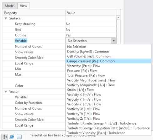
display.pref = flow.P - 101325
#display.pref: Gauge Pressure [Pa]
When you use these expressions, the Gauge Pressure entity appears under the values for the Variable property as shown below.
Variables at Monitoring Points
You can access the local cell variables at any monitoring point using the following format:
module[.subname][email protected]
Point coordinates:
probe.coord@probe_name
Example:
inletP = flow.P@probe."Point01"+101325
User defined variable for XY-Plot
plot.varname — Defines a user variable that you can use in XY Plots. The New Common variable is added as a value for the Variable property in the Properties Panel.
#plot.varname: dispname [unit] — (Optional) Defines a new name with unit for a user defined variable.
Example:
plot.head = (flow.pt@outlet - flow.pt@inlet)/998/9.8
#plot.head: Pressure Head[m]
• Do not add a space before the colon symbol when you define a new display or plot variable name and unit. • Default units for display and plot variables appear in square brackets. For example, the default unit Pa appears for the pressure variable. If you define a unit properly, the unit appears on the screen. In this example, when you change the final unit that appears, its values are also converted. If you do not define the unit properly, the software ignores the unit. |
Other functions
Expression Operators | Function | Example |
|---|---|---|
abs(x) | absolute value function | |
max(x,y) | maximum function | a = max(b,c) ==> a= b if b >c or a=c if c>=b |
min(x,y) | minimum function | a = min(b,c) ==> a= b if b <c or a=c if c<=b |
mod(x,y) | modulus function | a = mod(c,b) ==> a = the remainder of c divided by b |
sgn(x) | returns a flag (-1, 0, or 1) indicating the sign | a= sgn(b) ==> a = -1 if b<0 a = 0 if b=0 a = 1 if b>0 |
step(x) | step function returns a 0 or 1 depending on the value relative to zero | a= step(b) ==> a = 0 if b<0 a = 1 if b>=0 |
Tables
The table function enables the inclusion of data from external table files located in the same directory as the project file (*.spro).
Table Expressions | Function |
|---|---|
table(filename,x) | Interpolates from a 1-D Table |
table(filename, x ,y) | Interpolates from a 2-D Table |
Example:
Using tables:
# Extracting information from tables
p = table("inlet_pressure.txt",time)
density = table("R134a_density.txt",temp,pre)
• Table Format: 1-D (filename,x)—Allows you to access a 1-D data table located in the same directory as the project file (*.spro).
◦ 1-D Table for Uniform Distribution Format
<?xml version="1.0" encoding="ISO-8859-1"?>
<table size="n" min="xmin" max="xmax" outside="flat | extrapolation">
# comments (x assumed to have uniform distribution)
v1
v2
...
vn
</table/>
<table size="n" min="xmin" max="xmax" outside="flat | extrapolation">
# comments (x assumed to have uniform distribution)
v1
v2
...
vn
</table/>
◦ 1-D Table for Non-Uniform Distribution Format
<?xml version="1.0" encoding="ISO-8859-1"?>
<table size="n" outside="flat | extrapolation">
# You can add comments by putting the hashmark “#” in front .. but do not insert comments before the xml line (line 1)
x1 v1
x2 v2
xn vn
</table/>
<table size="n" outside="flat | extrapolation">
# You can add comments by putting the hashmark “#” in front .. but do not insert comments before the xml line (line 1)
x1 v1
x2 v2
xn vn
</table/>
In the format, outside = “flat” or outside = "extrapolation" under the table tag determines how you determine a value when the input x, y is out of range.
• Table Format: 2-D (filename,x)— Allows you to access a 2-D data table located in the same directory as the project file (*.spro).
◦ Format of the 2-D Table for Uniform Distribution
<?xml version="1.0" encoding="ISO-8859-1"?>
<table size="nx my" min="xmin ymin" max="xmax ymax" outside="flat | extrapolation">
# comment
# values table (x and y assumed to have uniform distribution
v(x1,y1) v(x2,y1) … v(xn,y1)
v(x1,y2) v(x2,y2) … v(xn,y2)
...
v(x1,ym) v(x2,ym) … v(xn,ym)
</table>
<table size="nx my" min="xmin ymin" max="xmax ymax" outside="flat | extrapolation">
# comment
# values table (x and y assumed to have uniform distribution
v(x1,y1) v(x2,y1) … v(xn,y1)
v(x1,y2) v(x2,y2) … v(xn,y2)
...
v(x1,ym) v(x2,ym) … v(xn,ym)
</table>
◦ Format of the 2-D Table for Non- Uniform Distribution
<?xml version="1.0" encoding="ISO-8859-1"?>
<table size="nx my" outside ="flat | extrapolation">
# x and y variable ranges
x1 x2 … xn
y1 y2 … ym
# values table
v(x1,y1) v(x2,y1) … v(xn,y1)
v(x1,y2) v(x2,y2) … v(xn,y2)
...
v(x1,ym) v(x2,ym) … v(xn,ym)
</table>
<table size="nx my" outside ="flat | extrapolation">
# x and y variable ranges
x1 x2 … xn
y1 y2 … ym
# values table
v(x1,y1) v(x2,y1) … v(xn,y1)
v(x1,y2) v(x2,y2) … v(xn,y2)
...
v(x1,ym) v(x2,ym) … v(xn,ym)
</table>
In the format outside = “flat” or outside = "extrapolation" under the table tag dictates how to determine a value when the input x, y is out of the range.
To add a comment, put a hash-mark “#” before the text. Do not insert comments before the xml line or line 1. |