Using the Results Legend in Creo Simulation Live
About the Results Legend
The results legend is used for the following:
• To select the result quantity to display.
• To select the units of the result quantity to display.
• To select the component of the result.
• To select the result rendering method.
• To vary the range of results displayed.
• To select the mode and view the corresponding frequency in the case of a modal analysis.
• To view simulation time for flow and transient thermal studies.
The following figure illustrates the use of the results legend. In this example the result quantity selected is velocity. The maximum value of velocity that is displayed is 132530 (1.3253 e05) mm/sec which is the global maximum , and the minimum value is zero which is the global minimum for the simulation study. You can vary the values in the legend between the global maximum and minimum values.
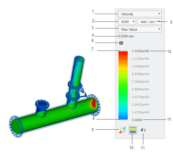
1. Selects a suitable result quantity from the list.
2. Selects a component of the result quantity where applicable —for example velocity, deformation.
3. Selects a suitable result rendering method based on the results you want to view.
4. Displays the simulation time. It is only applicable to transient thermal and transient fluid simulation studies.
5. Units—Selects appropriate units for the result quantity displayed.
6. Collapses or expands the legend.
7. Pull the top edge of the legend downward to change the range of the maximum result value that is displayed in the model. Double-click to edit the maximum value for the displayed range.
8. Pull the bottom edge of the legend upward to change the range of the minimum value displayed. Double-click to edit the minimum value for the displayed range.
9.  —Toggles the display of the location of the minimum and maximum values of the result quantity in the graphics window. The location is shown as red and blue circles.
—Toggles the display of the location of the minimum and maximum values of the result quantity in the graphics window. The location is shown as red and blue circles.10.  —Toggles between displaying results as distinct color bands or as diffused colors. Display shows diffused colors by default.
—Toggles between displaying results as distinct color bands or as diffused colors. Display shows diffused colors by default.11.  —Resets the legend range to the global maximum /minimum.
—Resets the legend range to the global maximum /minimum.12. Double-click and type a value for the maximum value to be displayed.
13. Double-click and type a value for the minimum value to be displayed.
Result Quantities
Some of the result quantities that are calculated for a study are also available in the legend. The types of result quantities available depend on the active simulation study. When you change the selected result type, the results that appear in the graphics window change instantly. Some result quantities can be queried as probes even though they are not available in the Results legend. The following result types are available for a study:
Study Type | Available in Legend | Result Type | Description | ||
|---|---|---|---|---|---|
Modal |  | Modal Frequency | Frequency response of the model for the selected mode. | ||
Modal, Structure | | Deformation | Deformation of the model—either total or in a specific direction. | ||
Structure | | Von Mises Stress | A combination of all stress components. | ||
Structure | | X Normal Stress | Normal stress along the X-axis. | ||
Structure | | Y Normal Stress | Normal stress along the Y-axis. | ||
Structure | | Z Normal Stress | Normal stress along the Z- axis. | ||
Structure | | XY Shear Stress | Shear stress acting in the Y- direction on the plane whose outward normal is parallel to the X- axis. | ||
Structure | | YZ Shear Stress | Shear stress acting in the Z- direction on the plane whose outward normal is parallel to the Y axis. | ||
Structure | | XZ Shear Stress | Shear stress acting in the Z- direction on the plane whose outward normal is parallel to the X axis. | ||
Structure | | Maximum Principal Stress | Maximum principal stress. | ||
Structure | | Middle Principal Stress | The principal stress that has a numerical value between maximum principal and minimum principal. | ||
Structure | | Minimum Principal Stress | Minimum principal stress. | ||
Structure | | Local Reaction Force | A reaction force that develops at constrained locations in a model. | ||
Structure | | Reaction Resultant | The sum of all reaction forces. | ||
Fluid Simulation | | Velocity | Flow velocity in a fluid simulation study. | ||
Thermal | | Temperature | Temperature distribution in a fluid simulation study or thermal study. | ||
Thermal | | Heat Flux | Heat flux results for a fluid simulation study or thermal study | ||
Thermal, Conjugate heat transfer mode of Fluid Simulation |  | Heat Flow | Heat flow through a solid. | ||
Fluid Simulation | | Static Pressure | The pressure at a point on a body moving with the fluid. | ||
Fluid Simulation | | Total Pressure | The sum of static and dynamic pressure. | ||
Fluid Simulation | | Vortices | For a fluid simulation study, vortices show the region in a fluid in which the flow revolves around an axis line, which may be straight or curved. | ||
Fluid Simulation | | Force X | Force in the X- direction on the surface of a fluid body. | ||
Fluid Simulation | | Force Y | Force in the Y- direction on the surface of a fluid body. | ||
Fluid Simulation | | Force Z | Force in the Z- direction on the surface of a fluid body. | ||
Fluid Simulation | | Mass Flow | A measure of the mass flow rate. | ||
Fluid Simulation | | Volume Flow | A measure of the volumetric flow rate. | ||
| |||||
Result Rendering Method
Rendering Method—Selects the result rendering method used to generate the result image in the graphics window:
• Surface—Shows you the results on the surface of the model.
• Composite—Views activity inside the model.
• Inverse Surface—See behind the first surface encountered in the model from a specific viewpoint. This is referred to as surface skipping. This technique gives you a better understanding of the underlying structure of complicated models.
• Isosurface—Visualizes the surfaces that correspond to a specific value of a quantity.
• Max Value—Displays the maximum value of a quantity found along a line of sight drawn from your eye to the back of the model. This method is useful when trying to find maxima in the model that might be otherwise obscured.
• Min Value—Displays the minimum value found along a line of sight drawn from your eye to the back of the model.
Result Component
Result Component—Choose the vector component of the result that you want to display:
• X—X- component of result quantity.
• Y—Y- component of result quantity.
• Z—Z- component of result quantity.
• SUM—The resultant value of the result quantity.
Varying the Range of Results Displayed
You can use the results legend to vary the range of results displayed.
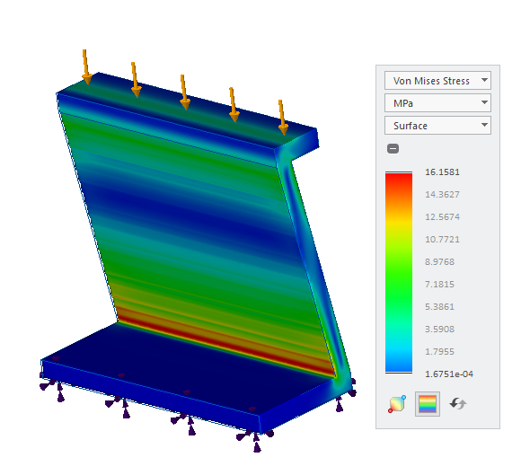
In the following example of Von Mises stress, the default values on the results legend are as shown in the following figure. The maximum value (16 MPa) on the legend is the global maximum and the minimum value is close to zero, and is the global minimum value.
Set the upper limit to 10 MPa and the lower limit to 0. The results are as shown below.
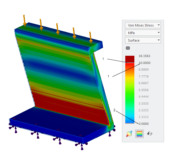
1. Double click and specify 10.000 or pull to make the upper limit 10.000
2. Double-click and type an exact value – 0 as the lower limit of the legend.
All the results above 10MPa are displayed in red and all results below 0 are blue.
Click to reset the legend limits to the default value.
to reset the legend limits to the default value.For the same simulation you can view results in a narrower range, for example to view stresses between 5 and 10 MPa, double-click the minimum value and type 5, and double-click the maximum value and type 10. The range of results is now from 5 to 10 MPa as shown in the following figure.
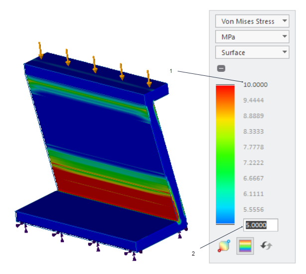
1. Double-click and type the maximum value 10 MPa or pull to adjust the upper limit.
2. Double-click and type the minimum value 5 MPa or pull to adjust the lower limit.