Read the problem defined below, and then, in Task 3–1 through Task 3–3, find the solution using the following methods:
• State-Space ODE solver
• ODE solver
• Solve block
Problem Definition
Consider the classical mass-spring-damper system:
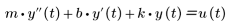
The dynamical equation for this system is given by the following equation:
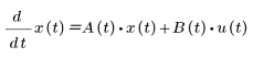
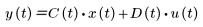
You can represent this system with a state-space model expressed in the following form:
Where:
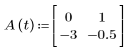
• A—State matrix
• B—Input matrix
• C—Output matrix
• D—Direct transmission matrix
• x—State vector
• u—Input
• y—Measured or controlled output
You can obtain the linear system above by linearizing the state and the output nonlinear equations that model the system dynamics.
Use two state variables for this second order system.
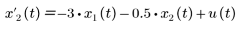
Given that m = 1, b = 0.5, and k = 3, the system equations are as follows:
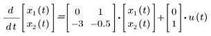
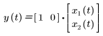
In a state-space matrix form, the model is written as follows:
State-Space ODE Solver
1. Define the matrix functions A, B, C, and D.
2. Define the input to be the heaviside step function. To insert the step function, type F, and then press Ctrl+G.
3. Define the initial condition of the two variables. To type i as a literal subscript, on the Math tab, in the Style group, click Subscript, and then type i.
4. Define time boundaries over which you want to find the system solution.
5. Define the number of points at which you want to find the solution, excluding ti.
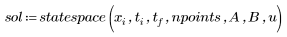
6. Call the statespace function.
The first column of matrix sol contains the time at which the solution is found. Its remaining columns contain the state variables x1 and x2 at that time.
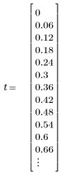
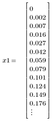
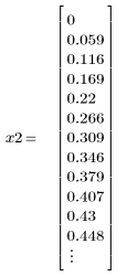
7. Extract t, x1, and x2 from matrix sol.
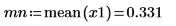
8. Calculate the mean and maximum values of x1.
9. Plot x1 over time and use markers to show its mean and maximum values.
The plot shows the transient response characteristics such as the rise time, the overshoot, and the settling time.