In the previous task, you solved the mass-spring-damper system with a state-space ODE solver. You can also use ODE solvers to solve this problem. Recall that the dynamical equation was as follows:
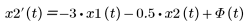
The system parameters were m = 1, b = 0.5, and k = 3. The input was a heaviside step function, u(t) = Φ(t). You can rewrite the second-order equation in terms of first-order ODEs:
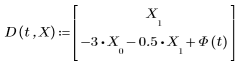
1. Define a vector function specifying the right side of the system.
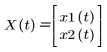
The arguments of D are t, the independent variable, and X, the vector of dependent variables:
2. Define the initial values for x1 and x2.
3. Define the initial and the final times over which to evaluate the solution.
4. Define the number of time steps.
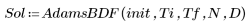
5. Call the AdamsBDF solver to evaluate the solution.
◦ The AdamsBDF solver is a hybrid solver. It starts with the non-stiff Adams solver. If it identifies the problem as stiff, it switches to the stiff BDF solver.
◦ Alternatively, you can replace the AdamsBDF solver by another ODE solver. For more information refer to the About Differential Equation Solvers topic in the Help.
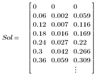
◦ The solution is a 3-column matrix with the time, the displacement, and the velocity of the system for each of the N steps:
6. Extract the time and the displacement from Sol and plot them one against the other.
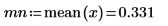
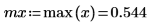
7. Calculate the mean and maximum values of x.
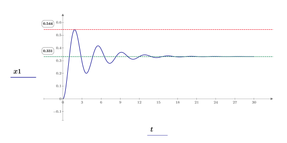
8. Plot x over time and use markers to show its mean and maximum values.
The plot shows the transient response characteristics such as the rise time, the overshoot, and the settling time.