Special Considerations of Volume of Fluid (VOF) Model
VOF Model versus Mixture Model
In the homogeneous Eulerian multiphase modeling approach, both the volume of fluid (VOF) and Mixture Eulerian models solve the same set of mixture (averaged) governing equations. However, they are based on different physical mechanisms and apply to different multiphase flow regimes:
• Mixture Model—Designed for two or more phases (fluid or particulate), which are treated as interpenetrating continua. It solves for the mixture momentum equation and energy equations and the phase-to-phase interface is not tracked or no clear interfaces are observed. Applications of the mixture model include particle-laden flows with low loading, bubbly and droplet flows, sedimentation, and cyclone separators. You can also use the mixture model with prescribed relative velocities for the dispersed phases to model inhomogeneous multiphase flows.
• VOF Model—Generally a transient surface-tracking technique designed for two or more immiscible fluids where the position of the phase-to-phase interface is of interest. In the VOF model, a single set of mixture momentum and energy equations is shared by all the phases and solved implicitly. The phase volume fractions are obtained using accurate explicit or implicit time algorithms with higher-order advection schemes to resolve sharp interfaces between a pair of phases. Typical applications of the VOF model include stratified flows, free-surface flows, filling, sloshing, the motion of large bubbles in a liquid, the motion of liquid after a dam break, the prediction of jet breakup (surface tension), and the tracking of any liquid-gas interfaces.
The VOF formulation relies on the fact that two or more fluids (or phases) are not interpenetrating. In any given control volume cell, therefore, the local phase volume fractions can alone determine whether it contains only one of the phases, or a mixture of phases. For instance, for the qth phase, if the volume fraction in a cell is αq, then only the following three conditions are possible:
◦ αq = 0: The cell is empty of the qth phase
◦ αq = 1: The cell is full of the qth phase
◦ 0< αq < 1: The cell contains the interface between the qth phase and one or more other phase.
Therefore, you can accomplish the tracking of the interfaces between the phases from the solution of a transport equation for the volume fraction of one or more of the phases.
The Effect of Surface Tension
Surface tension is the elastic tendency of a fluid surface which makes it acquire the least surface area possible. Consider an air bubble in a liquid. Within the bubble, the net force on a molecule due to its neighbors is zero. At liquid-air interfaces, the surface tension results from the greater attraction of liquid molecules to each other due to cohesion than to the molecules in the air due to adhesion. The net effect is a radially inward force at its surface, which makes the bubble contract. The pressure inside the bubble increases to counterbalance the intermolecular attractive force.
• The Continuum Surface Force Model
In
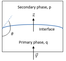
Creo Flow Analysis, the VOF model can include the effects of surface tension along the interface between each pair of phases. The surface tension model adopted is based on the Continuum Surface Force (CFS) model of Brackbill et al. This approach considers the surface tension effect as an additional volumetric force concentrated at the interface, rather than a surface force. For the free surface interface shown in
figure 2.26, the primary fluid is phase q (the liquid phase), and the secondary fluid is phase p (usually a gas phase). According to the continuum surface force model, the surface curvature is computed from local gradients in the surface normal at the interface. Let

be the surface normal vector, defined as the gradient of the primary fluid volume fraction, α
q:
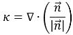
The interface curvature k, is defined in terms of the divergence of the unit normal vector:
equation 2.93
where

is the magnitude of the vector
.
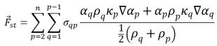
The surface tension force at the surface is expressed as a volumetric force using the divergence theorem, which is an additional source term added to the mixture momentum equation:
equation 2.94
where σ
qp is the surface tension coefficient between fluid q and fluid p. It has the unit of N/m.
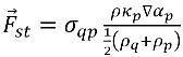
Equation 2.94 allows for a smooth superposition of forces near cells where more than two phases are present. If only two phases are present in a cell, you have the following relations:
equation 2.95
equation 2.96
• Including the Surface Tension Force
The importance of surface tension effects is determined by two nondimensional parameters: the Reynolds number Re and the capillary number Ca, or the Reynolds number and Weber number We:
If Re<<1, the parameter of interest is the capillary number:
equation 2.97
where U∞ is the free-stream velocity. The surface tension effects are neglected if Ca>>1, since the surface tension force is too small.
If Re>>1, the parameter of interest is the Weber number:
equation 2.98
where L is the characteristic length. The surface tension effects can also be neglected if We>>1, when the inertial force is much larger than the surface tension force.
Wall Adhesion (Contact Angle)
The volume of fluid (VOF) model has an option to specify a wall adhesion angle in conjunction with the surface tension model. According to Brackbill et al., instead of the application of this boundary condition at the wall directly, the contact angle between the fluid and wall at the interface is used to adjust the surface normal in cells near the wall. This so-called dynamic boundary condition results in the adjustment of the curvature of the surface near the wall.
If θ is the contact angle of the free-surface interface at the wall, as shown in
figure 2.26, then the unit normal vector at the near-wall cell is calculated as:
equation 2.99
where,
| unit vector normal to the wall |
| unit vector tangential to the wall |
Then the calculated unit normal velocity

is used to determine the local curvature of the surface,
equation 2.93, and subsequently the surface tension force,
equation 2.94, or
equation 2.95.