Simulation Example
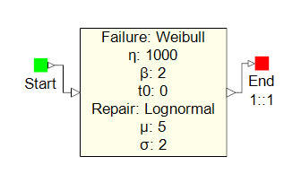
This simple simulation example demonstrates how to evaluate the time-specific availability of the one-component system shown below. All availability results are for the end time of a 1000-hour mission. Failure and repair properties are provided in the figure.

Under RBD in the Calculate window, on the General page, Availability is selected. On the Advanced page, Force Monte Carlo simulation is selected, Number of simulation iterations is set to 1000, and Specify random number seed is set to 1. Using these values and the defaults for all other parameters, the result calculated for availability is 0.727. Is this the true value for availability? To answer this question, set Specify random number seed to 2 and recalculate. The availability result is 0.75, which is a difference of 0.023.
The answer varies with the seed because the sequence of random numbers used in the simulation process is different. So, what is the true value of availability? Remember that simulation produces accurate results only when the number of iterations is large. When this is the case, the result does not depend on the seed because all possible sequences of random numbers produce the same availability value.
If you set Number of simulation iterations to 10,000,000 and Specify random number seed to 1, when you recalculate, the availability result is 0.736208. If you set Specify random number seed to 2 and recalculate, the availability result is 0.736297. The difference in results is 0.00089, which is much less than 0.023. In general, the difference decreases as the number of iterations increases. However, increasing the number of iterations increases the computational time. In general, these increases are directly proportional. This means that increasing the number of iterations by 100 increases the computational time by a factor of 100.
The effects of randomness on the results can be measured with the variance of the simulation output and the confidence intervals on the availability results. The confidence intervals are the range of availability values, bounded above and below, within which the true availability value is expected to fall with a certain percentage of confidence. The width of the confidence intervals is directly proportional to the standard deviation (square root of the variance). The standard deviation is inversely proportional to the square root of the number of simulations.
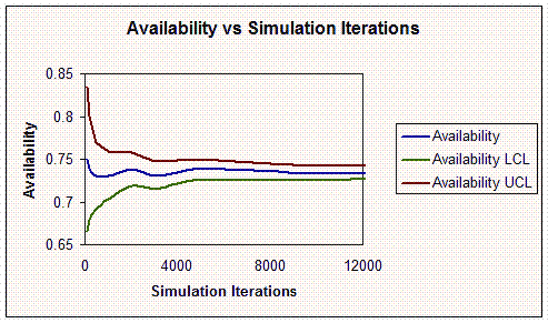
For example, increasing the number of simulation iterations by four times generally reduces the standard deviation to approximately 50%. Hence, the width of the confidence intervals is reduced by 50%. Reducing the standard deviation also decreases the width of the confidence intervals. Therefore, the number of iterations can be adjusted so that the confidence intervals are within the required accuracy. The following diagram shows this relationship.

Assume that you want to find the availability of this single-component system within ± 1% accuracy with a 95% confidence. First, reset Number of simulation iterations to 1000, and Specify random number seed to 1. Then calculate availability and 95% confidence intervals. The results are:
• Availability = 0.727
• Availability LCI = 0.699382
• Availability UCI = 0.754618
The width of the confidence interval for availability is UCI − LCI (0.055236). The width is 7.6% of the availability (0.727). If the true value falls somewhere within this interval, then the maximum possible error is ± 3.8% of the availability.
The true value falls within these bounds with a 95% confidence. Therefore, the maximum possible error in the availability results is ± 3.8% with 95% confidence. It is 3.8 times the required accuracy of ± 1%. To reduce the width of the intervals 3.8 times, you must increase the number of simulations to (3.8)2 or approximately 14 times.
Thus, compute the results with 14,000 simulations. The results are:
• Availability = 0.732143
• Availability LCI = 0.724806
• Availability UCI = 0.73948
The width of the interval is 0.014674. It is 2.0% of the availability estimate. Therefore, the maximum possible error is ± 1% with 95% confidence. This procedure provides a quick way to determine the number of simulation iterations to use.