Confidence Intervals
The Chi-square (χ 2) distribution can be used to find the confidence intervals on the failure rate (λ) and the MTTF (mean time to failure) of exponential distributions. The χ 2 distribution can also be applied to the Weibull distribution when the shape parameter (β) is known (WeiBayes method). This topic presents the formulas that are specific to exponential distributions.
The estimate for failure rate ( ) is calculated as the ratio of the number of failures and total testing time. Even though it is the best available estimate, it by itself gives no measure of precision or risk. If critical decisions depends on the true value of , ask the following important questions:
) is calculated as the ratio of the number of failures and total testing time. Even though it is the best available estimate, it by itself gives no measure of precision or risk. If critical decisions depends on the true value of , ask the following important questions:• Can the true λ be as high as 10 * λ?
• Are we confident it is no worse than 1.2 * λ?
• How much better than might the true λ be ?
might the true λ be ?When critical decisions are being made, confidence intervals should be used. For type I (time-censored) or type II (failure-censored at the rth failure) data, factors based on the χ 2 distribution can be derived and used as multipliers of to obtain the upper and lower ends of the confidence interval. The remarkable thing about these multipliers is that they depend only on the number of failures observed during the test (or in the field).
to obtain the upper and lower ends of the confidence interval. The remarkable thing about these multipliers is that they depend only on the number of failures observed during the test (or in the field).Suppose we want a 100 (1 − α) confidence interval for λ, where α is the risk we are willing to accept that our interval does not contain the true value of λ. For example, α = 0.1 corresponds to a 90% interval. We can calculate a lower 100 (α / 2) bound for λ and an upper 100 (1 − α / 2) bound for λ. These two numbers give the desired confidence interval. When α = 0.1, this method sets a lower 5% bound and an upper 95% bound, having between them a 90% chance of containing the true λ. However, in some applications, we may be interested in only one-sided bounds.
For type II censoring data (at r th failure), follows the chi-square distribution with 2r degrees of freedom. It follows that:
follows the chi-square distribution with 2r degrees of freedom. It follows that: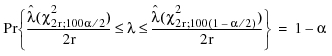
For type I censored data (time-censored), intervals using the above factors are approximately correct. Exact intervals can be calculated only if failed units are immediately replaced during the course of the test. In this case, the lower bound factor is exactly as above, while the upper bound factor uses the 100 (1 − α /2) percentile of a χ2 with 2(r + 1)degrees of freedom, still divided by 2r. It should be noted that this χ2 factor produces a slightly more conservative upper bound. Therefore, we recommend using it only for type I censored data. The probability statement is as follow:

Using this for type I censoring without replacement gives an upper bound equivalent to assuming that another failure has occurred exactly at the end of the test and that we had type II censoring (failure censoring) with r + 1 failures.
Similarly, we can calculate one-sided bounds. For example, the one-sided upper bound for type II censoring (failure censoring) is:
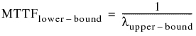
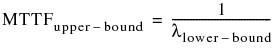
Because MTTF is the reciprocal of the failure rate, the lower and upper bounds for MTTF can be obtained by using the upper and lower bounds of the failure rate: