Analysis
Many studies have been carried out to display the effects of operational scenario on the achieved reliability of complex electronic systems, and many attempts have been made to empirically derive correction factors that can be applied to the results of predictions. Although the derived mathematical models differ in form and correction factors, the research leading to their derivation shares a common thread.
The generally accepted belief is that the damaging effects of cyclic operations can be attributed to a complex combination of electrical and thermal stress, moisture ingress, physical shock, airborne corrosive agents and transient power surges. There is also empirical evidence to suggest that the way these factors combine may produce a progressively degenerative effect that systematically reduces a system's ability to withstand the increased stress of cyclic operation.
Before an attempt to derive some meaningful correction factors can be made, those parameters that are fixed in the prediction process but subject to significant variation in service must first be identified. Varying the baseline temperature used for the prediction can mitigate thermal effects and account for major environmental differences.
Mission profile is the main area not addressed. Both the number of missions and the mission duration are normally assumed to be constant for a prediction. Indeed, most models assume constant operation. An attempt must therefore be made to correct for:
• Variation from the 100% usage factor.
• The number of power on/off cycles.
• Variation in mission duration.
MIL-HDBK-217 assumed that the constant random failure rate is modified by the effect of on/off cycling to some extent, but by far the most significant is the effect of mission duration. For a given number of power cycles the increase in failure rate will be relatively constant, whereas the calculated reliability will vary with mission duration.
Example Failure Rate Variations Due to Mission Duration Versus Calculated Reliability
1. Assume 10 missions during which there are a total of 6 failures, 5 attributed to the constant random failure rate and 1 attributed to the increased power cycling. Experience shows that the failure rate does not vary significantly with mission duration but calculated reliability certainly does:
◦ If each mission is of 24 hours duration, then:
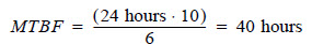
◦ If each mission is of 500 hours duration, then:

2. When lower one-sided statistical confidence limits using the Chi-squared distribution are applied, this difference becomes even more pronounced:
◦ If each mission is of 24 hours duration, then:
▪ 90% lower, one-sided confidence gives 23 hours.
▪ 80% lower, one-sided confidence gives 26 hours.
▪ 70% lower, one-sided confidence gives 30 hours.
◦ If each mission is of 500 hours duration, then:
▪ 90% lower, one-sided confidence gives 475 hours.
▪ 80% lower, one-sided confidence gives 551 hours.
▪ 70% lower, one-sided confidence gives 616 hours.
Much work has been carried out in this area, and one example is documented by the Reliability Analysis Centre, Rome Laboratory, Griffiss Air Force Base, New York. (RADC-TR-89-299: Reliability and Maintainability Operational Parameter Translation II). The model developed for ground-based equipment is:
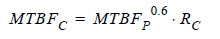
Where:
MTBFC = The corrected value of operational reliability.
MTBFP = The predicted inherent reliability.
RC = The reliability correction factor (4.8 for mobile systems and 27 for fixed systems).
Empirical testing of this model against real-world observations has shown it to be reasonably representative; but, in many cases, it is still too coarse, having only two possible outcomes, as can be seen in the next example.
Example Real-World Scenarios
MIL-HDBK-217 parts stress prediction carried out for 30°C in a ground fixed environment gives an MTBF of 600 hours. This equipment is deployed in three distinctly different scenarios and is exhibiting a similar number of different levels of reliability performance.
Scenario 1: Training Role (Potentially Mobile)
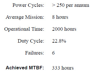
Scenario 2: Gap Filler Role (Mobile)

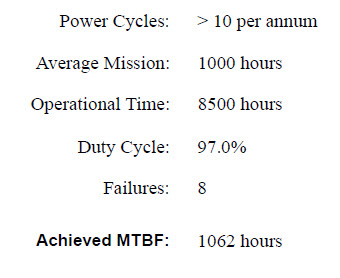
Scenario 3: Fully Operational Role (Fixed Site)
Using the RAC parameter translation models:
• For scenarios 1 and 2, the result is 223 hours.
• For scenario 3, the result is 1235 hours.