This topic provides a workaround for two cases of non-convergence errors when numerically evaluating integrals with one or two infinite integration limits.

To explain the two cases, define a mean μ and a standard deviation σ.

Set multiplier variable n to 1, and then define function g(x) in terms of the built-in probability density function dnorm.

When n=1, evaluating the integral of g(x) over the range [0, ∞] does not return an error, but returns a very small value.

Increase the value of n to n=2 and re-evaluate the integral.

Increasing the value of n to n=2 results in an error because the calculation is not converging to a solution.

As a workaround, set variable T to a value that is close to the tail of g(x), and then split the single integral into two: one that covers range [0, T] and one that covers range [T, ∞].

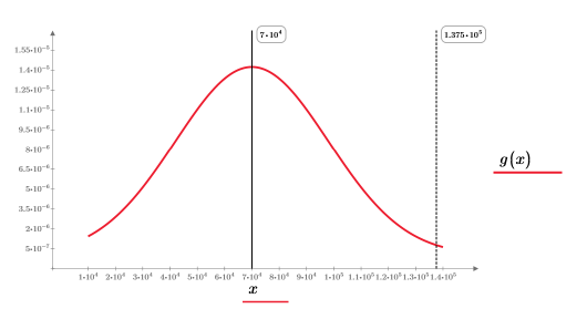
The split integral A3 returns a good answer when n=1 or n=2. Plot g(x) and add vertical marker T to see how close it is to the tail of g(x).

The plot shows variable T as the vertical marker close to the tail of g(x).

Set the multiplier variable n to 1, and then evaluate the integral of g(x) over the range [-∞, ∞].

When n=1, evaluating the integral of g(x) over the range [-∞, ∞] returns no error but the returns a very small value.

As a workaround, set variables T1 & T2 to values that are close to the head and tail of g(x), and then split the single integral into three integrals: one to cover range [-∞, T1], one that covers range [T1, T2], and one that covers range [T2, ∞].

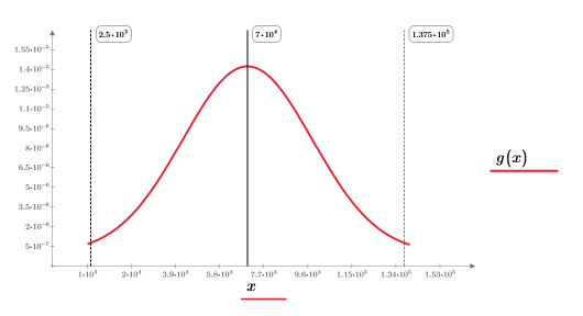
The split integral returns a good answer when n=1 or n=2. Plot g(x) and add vertical markers T1 and T2 to see how close they are to the head and tail of g(x).

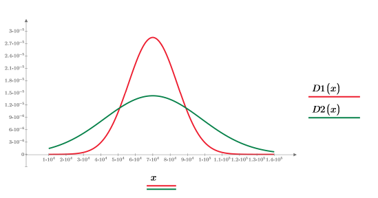
Plot the built-in probability density function dnorm using the same mean but two different values of standard deviation.

The plot shows that:

In both cases, splitting the integral ensures that the calculation converges and returns the correct answer.