Example: The Chirp z-Transform
The chirp z-transform takes the spectrum of a sampled signal and interpolates at uniformly spaced frequency values over a small frequency interval.
The algorithm used is the chirp z-transform described in Samuel Stearns and Ruth David, Signal Processing Algorithms (Prentice-Hall, Inc.).
Creating the Signal
1. Define the signal frequencies.


 |  |  |
 | ||
The decaying sine wave signal is the product of an exponential function that decays to zero with time and a sine wave function.
3. Plot the decaying signal.
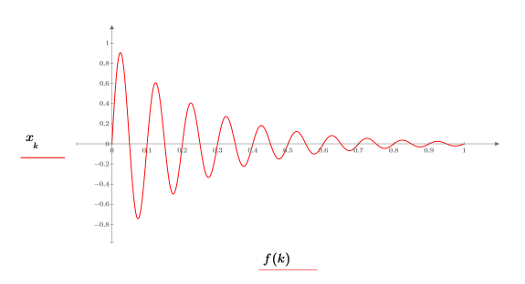
The frequency is normalized so that 1 represents the sampling frequency.


5. Plot the DFT of the signal. Use vertical markers to show the magnitude and frequency of the first peak.

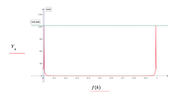
The peak occurs at the frequency of the sine wave, convolved with the spectrum of the exponential.
6. Zoom in on the first peak by expanding the frequency scale along the x-axis.
 |  |  |
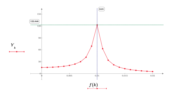
7. Calculate the number of data points inside the frequency range.

chirpz
Use the chirpz function to get a closer look at the spectrum around the peak by increasing the number of data point.
1. Set the step parameter and use the chirpz function to compute the spectrum.


2. Calculate the number of points in the interpolated spectrum.


3. Super impose the first peak of the DFT and the interpolated spectrum using the new range.
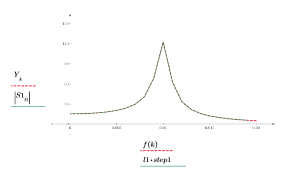
A step of 0.001 yields the same number of data points in the chirp-z trace and thus the two traces appear to be identical.
4. Reduce the step size 10 folds, and then recalculate and replot the two functions.


5. Calculate the new number of points in the interpolated spectrum.


6. Super impose the first peak of the DFT and the newly interpolated spectrum.
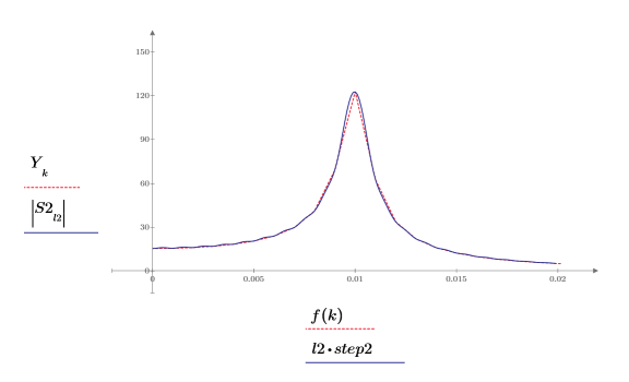
The plot shows that as the number of interpolated points increases, the spectrum trace becomes more rounded around the peak.
7. Reduce step2 by another 10 folds and observe its effect on the above plot.