Example: FIR Filter Design
Lowpass Filter Window Comparison
Calculate the coefficients for a low pass filter using two different windows, rectangular and Blackman.
1. Set the normalized cutoff frequency and number of coefficients.


2. Use the lowpass function to calculate the coefficients with rectangular and Blackman windows.


3. Define a range for displaying the coefficients and computing the frequency response.

4. Plot the two sets of coefficients.
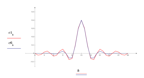
5. Use the gain function to calculate the gain of the frequency responses.


6. Use the phase and phasecor functions to calculate the magnitude and phase of the frequency responses.


7. Plot the magnitude of the frequency responses. Use a horizontal marker to mark the magnitude at the cutoff frequency.

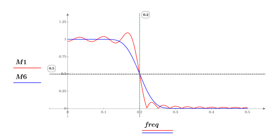
Both traces go through the cutoff frequency point, but M1 provides a sharper transition. The magnitude of either frequency response at the cutoff frequency is 0.5.
8. Plot the phase of frequency responses. Use a horizontal marker to mark the phase at the cutoff frequency.

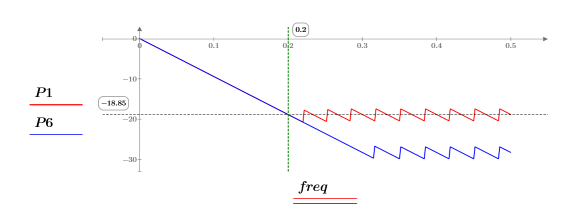
Both traces go through the cutoff frequency point. The phase of the frequency response at the cutoff frequency is -18.85.
9. Plot the dB magnitude of frequency responses. Use a horizontal marker to mark the dB magnitude at the cutoff frequency.

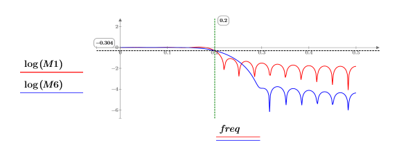
Both traces go through the cutoff frequency point. The dB magnitude at the cutoff frequency is -0.304.
Filtering by Convolution
Use convolution to apply these FIR coefficients.
1. Use the sin function to define a signal with low, middle, and high frequencies normalized with respect to the sampling frequency.
 |  |  |
 |  | |
 | ||
2. Plot signal x.
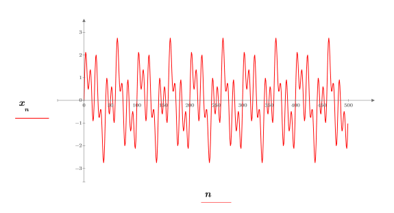
3. Use the lowpass, highpass, bandpass, and bandstop functions to generate filter coefficients using a Hamming window (number 5) and normalized filter cutoff frequencies.
 | |
 |  |
 |  |
 |  |
4. To filter the signal, convolve the filter impulse responses with x using function convolve for the first two and function response for the second two, demonstrating two approaches to this task.
 |  |
 |  |
5. Show that the output of convolve has a length equal to one less than the sum of the length of x and the coefficient array.


6. Plot the low pass output along with the low frequency component of the signal.


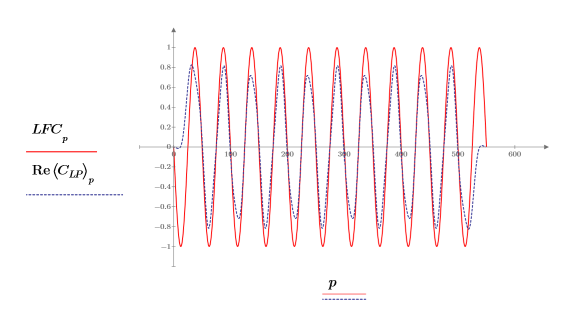
The sine wave is shifted to the right by 25 to allow for the delay introduced by the filter. The filter passes essentially only the low frequency, with some attenuation.
7. Plot the high pass output along with the high frequency component of the signal.

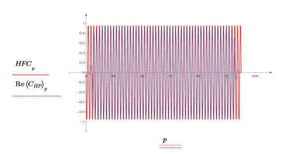
The sine wave is shifted to the right by 25 to allow for the delay introduced by the filter. The filter passes essentially only the high frequency, with some attenuation.
Checking the Effectiveness of Filters
1. Use the dft function to examine the effectiveness of the band stop filter by comparing the spectrum of the original signal with its spectrum after the filtering.


2. Plot the first 60 spectrum values of before and after filtering.


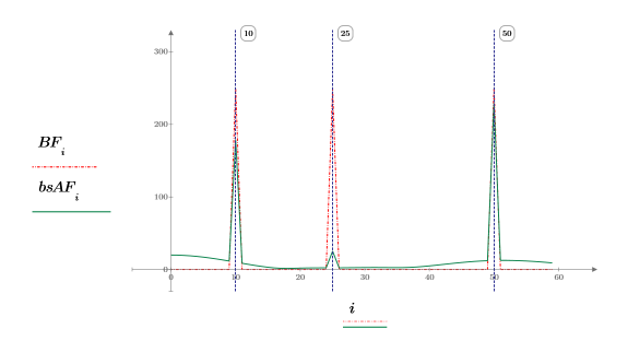
The middle frequency has been successfully attenuated.
3. Use the dft function to examine the effectiveness of the band pass filter by comparing the spectrum of the original signal with its spectrum after the filtering.


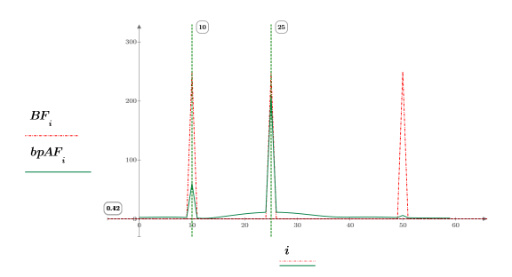
Most of the low frequency and all of the high frequency have been successfully attenuated.