Example: Filtering versus Exponential Smoothing
Compare the resulting smoothing achieved using the Detrending and Lowpass Filtering in the Transform Domain and the Time-domain Iterative Exponential Smoothing methods.
1. Define the number of data points.


3. Create a vector representing the time of each sample.


4. Use the slope function to get the slope of the line that best fits the signal, and then use the mean function to get the mean of the signal.


5. Plot the function and show its trend and mean lines.
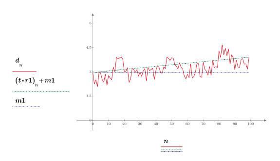
The mean line is horizontal while the trend line is not; indicating that the signal has a linear trend.
Detrending and Lowpass Filtering in the Transform Domain
The first step in smoothing by filtering is to remove the linear trend; otherwise, the transform displays frequency components of the linear signal, and not the higher frequency content.
1. Remove the trend from the signal. Recalculate the slope and the mean of the new signal.


2. Plot the new function and show its trend and mean lines.
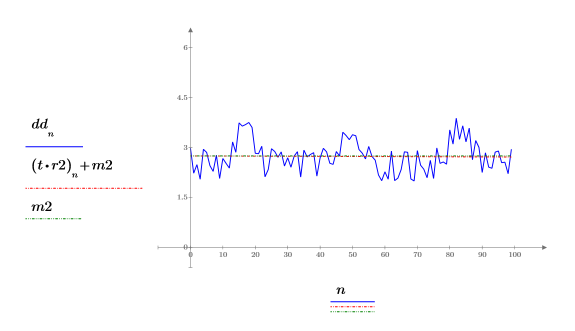
The mean and trend lines are horizontal; indicating that the signal has no linear trend.
3. Use the dft function to get the transform of the signal.

4. Window the transform by zeroing out the elements in the middle, saving only the beginning and the end, which represent the low frequencies.

5. Plot the windowed function. Use vertical markers to show the start and end of the window.
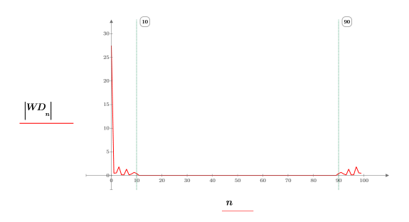
6. Use the idft function to get the inverse transform, and then add the trend back in.

Since vectors add element wise, the trend is added back using a single addition operator.
7. Plot the dw function.
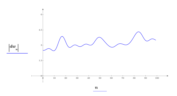
The trend has been restored to the smoothed function.
Time-domain Iterative Exponential Smoothing
Use the seeded iteration smoothing technique. To get seed values for the iteration, estimate the stationary and trend values, s and b, by looking at the beginning of the series.


2. Choose the two smoothing constants. The closer is α to 1, the more closely the smoothed curve tracks the original data.


Where P is the exponentially smoothed version of the original time series.
Compare the Two Techniques
Plot and compare the two smoothing techniques. The top two traces have been offset by 4 so that they can be displayed on the same graph.
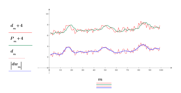
• The above traces correspond to the following types of smoothing (top to bottom): time series, exponential smoothing, time series, smoothed with a DFT.
• The exponential smoothing does not begin to track the data effectively until enough points have been averaged by the smoothing coefficients, a and b.
• Recalculate the worksheet and observe how the traces change due to having a different random number as part of the original signal definition.
• After each recalculation you can see that the DFT smoothed function tracks the original signal much better than the exponentially smoothed function.