Example: PDE in Solve Blocks
Use a partial differential equation (PDE) in solve block and the partial differential equation solver numol to compare solutions for a wave equation.
PDE Solve Block
To solve the following one-dimensional wave equation:

use the constraint:

To cast the first equation as a system of two partial differential equations, set up a PDE solve block


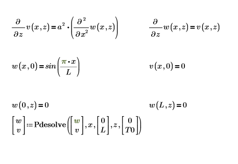
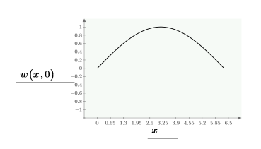
Here is a single solution on the boundary:
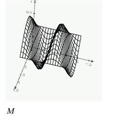
Create a grid of solutions to be plotted three-dimensionally with the CreateMesh function, using the constraints defined above:

Using numol
You can solve the command-line solver numol. This is especially useful when you want to include the calculation in a program.
Define the number of partial differential equations and algebraic constraints in your system:


The function for evaluating the right-hand side of the PDEs is a vector of length num_pde + num_pae (partial algebraic equations). In this case, the function is a system of equations. Similarly, the boundary condition is defined as a column vector of length num_pde + num_pae.
The expression for vector of PDEs:

Therefore, u1=v as defined above, and u0=w.
The vector of initial conditions:

Assume that each left-hand side is the first-order time derivative of the unknown function vector u. The function’s variables are x (space) and t (time). The solution is u, which can also be a vector of solutions for a system of equations: ux, the first derivative of each solution u in the vector, and uxx, the second spatial derivative.
You must use vector subscripts to address the individual entries in u, ux, and uxx.
The vector of boundary conditions can have three types of rows. Each row is determined by one of the following:
• rhs contains second-order spatial derivatives: two boundary conditions (either Dirichlet “D” or Neumann “N”) required, one for each side of the integration region.
• rhs contains first-order spatial derivatives: one Dirichlet boundary condition at left or right side of the integration region, the other is “NA”.
• If the vector contains no spatial derivatives, no boundary conditions are required.
Boundary conditions at the left and right borders, follow these conventions:


The result of numol is a matrix that represents each point in space as a row and each point in time as a column. This facilitates the visualization of solutions by allowing you to pick off one column at a time, representing the solution over all space at a single point in time. When solving a system of equations, the solution matrix for each unknown function is appended to the side of the previous matrix.


For the current example, there are 20 points in time for each function, so the matrix includes 40 columns. Pick the first solution, u0:


Comparing numol and Pdesolve
Compare numol and Pdesolve solutions at a point t0:
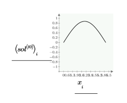
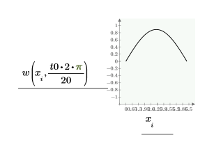
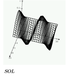
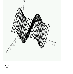
Compare the grid of solutions for the values of space and time:
