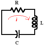
Given a simple electrical circuit containing a resistor R, an inductor L, and a capacitor C.
Use differential equations to model charge Q on capacitor C, then use ODE solver functions to find other approximate solutions. Finally, compare the results to the exact solution of Q.
Using Differential Equations
1. Write a differential equation for the voltage across the three components which must add up to zero:
2. Write the differential equation for the instantaneous change of charge Q on capacitor C:
3. Define charge Q at time zero:
4. Assume the following input parameter values:
5. Transform the differential equation into the standard form:
6. Solve the equation for all cases of a and b:
7. Plot the two possible solutions for Q:
Charge Q1 quickly decays to zero when a=b, and oscillates for a long time before reaching zero when a and b are not equal.
Before Using the ODE Solvers
• Define the parameters that will be passed to the ODE solver functions:
• The ODE solvers are divided into two types: solvers for stiff systems and solvers for non-stiff systems. A system of ODEs written in matrix form as y' = Ax, is called stiff if matrix A is nearly singular. Otherwise, the system is non-stiff.
• The distinction between stiff and non-stiff systems can be related to the inherent dynamics scales of matrix A as characterized by its eigen values. A matrix with disparate eigen values (or values ranging from too small to too large) is generally a stiff system.
• Based on the system parameters specified, this simple damped harmonic example represents a non-stiff system.
• Functions
Adams, AdamsBDF, BDF, and
Radau can be passed a specific value of TOL or use their own default TOL value of 10-5.
Using ODE Solvers for Non-Stiff Systems
Use the ODE solvers for non-stiff systems to find the approximate solutions, then compare the results to the exact solution of Q.
1. Adams
2. rkfixed
3. Rkadapt
4. Bulstoer
Using ODE Solvers for Stiff Systems
Use the ODE solvers for stiff systems to find the approximate solutions, then compare the results to the exact solution of Q.
1. BDF
2. Radau
Using ODE Hybrid solver
Use the ODE Hybrid solver AdamsBDF, which determines whether a system is stiff or non-stiff and calls Adams or BDF accordingly, to find the approximate solutions, then compare the results to the exact solution of Q.
1. AdamsBDF
Conclusion
• Within the ODE solvers for non-stiff systems, functions Adams and rkfixed return the solutions with the smallest and largest error, respectively.
• Within the ODE solvers for stiff systems, functions Radau and BDF return the solutions with the smaller and larger error, respectively.
• The hybrid function AdamsBDF returns a value that is smaller than both values returned by Adams or BDF.
• Overall, functions Radau and rkfixed return the solutions with the smallest and largest error, respectively.
Comparing Results
1. Plot the solutions returned by the ODE solvers for non-stiff systems with the smallest (Adams, G0nss) and largest (rkfixed, G1nss) errors:
There is a noticeable difference between the two returned solutions as compared with Q.
2. Plot the solutions returned by the ODE solvers for stiff systems with the smallest (Radau, G1ss) and largest (BDF, G0ss) errors:
The two solutions appear identical with respect to Q.
3. Plot the solutions, which yielded the smallest (Radau, G1ss) and largest (rkfixed, G1nss) errors, returned by the ODE solvers for stiff and non-stiff systems:
Function Radau, a stiff system solver, returns the best approximation to the solution of Q.