Cyclone Separator Exercise 7—Analyzing Results
This exercise describes how you analyze the results during and after the simulation. To hide CAD surfaces (not the fluid domain), switch between
 Flow Analysis Bodies
 and
 CAD Bodies
 in the
Show group. Click
 XYPlot Panel
 to view the XY Plot.
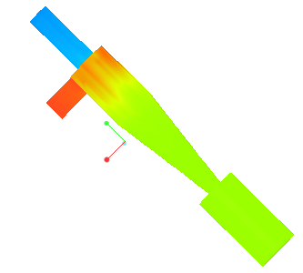
Viewing the Pressure Contours on a Boundary
In contours, physically equal values are connected by a curve.
| Pressure: [Pa] : Flow 101350.0 101320.0 |
1. In Boundary Conditions, under General Boundaries select CYCLONE_4_1_FLUID.
2. In the Properties panel, View tab, for Surface, set values for the options as listed below:
◦ Surface—Yes
◦ Grid—No
◦ Outline—No
◦ Variable—Pressure: [Pa] : Flow
◦ Min—101320
◦ Max—101350
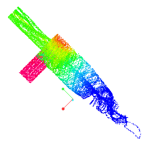
Viewing the Streamlines in the Domain
Streamlines track the path of fluid flow.
| Velocity Magnitude: [m/s] : Flow 5.95 0 |
1. Add Streamline01 to the Flow Analysis Tree and select it.
2. In the Properties panel, Model tab, set values for the options as listed below:
◦ Line Thickness—0.007
◦ Animation Time Size—0.0001
3. In the Properties panel, View tab, for Surface select the following values for the options listed:
◦ Variable—Velocity Magnitude: [m/s] : Flow
◦ Min—0.0
◦ Max—5.95
4. In the Flow Analysis Tree, under General Boundaries select BC_2.
5. In the Properties panel, Model tab for Streamline, set Release Particle to Yes.
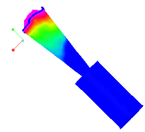
Viewing an Isosurface of Points with Velocity Below 1 m/s
In an isosurface, physically equal values are shown three-dimensionally in surfaces.
| Velocity Magnitude: [m/s] : Flow 1.000 0.00000 |
1. Click
 Flow Analysis
 >
 Isosurface
. A new entity
Isosurface 01 appears under
Derived Surfaces in the Flow Analysis Tree.
2. Select Isosurface 01.
3. In the Properties panel, Model tab, set values for the options as listed below:
◦ Isosurface Variable—Velocity Magnitude: [m/s] : Flow
◦ Type—Below Value
◦ Value—1.0
4. In the Properties panel, View tab, for Surface set values for the options as listed below:
◦ Variable—Velocity Magnitude: [m/s] : Flow
◦ Min—0.0
◦ Max—1.0
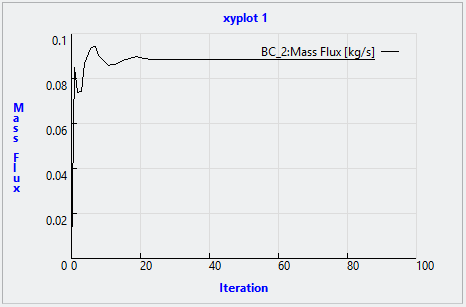
Plotting the Mass Flux at the Outlet Boundary
1. In the Flow Analysis Tree, under Boundary Conditions click General Boundaries.
2. Select BC_2.
3. Click
 XYPlot
. A new entity
xyplot1 is added in the Flow Analysis Tree under
Results >
Derived Surfaces >
XY Plots.
4. Select xyplot1.
5. In the Properties panel, set the Variable as Mass Flux.
6. Click
 Stop
Stop and
 Run
Run, if required.
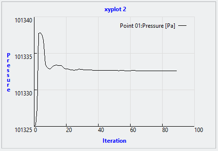
Plotting the Pressure at Monitoring Point
1. In the Flow Analysis Tree, under Results click Monitoring Points.
2. Select Point01.
3. Click
XYPlot. A new entity
xyplot2 is added in the Flow Analysis Tree under
Results >
Derived Surfaces >
XY Plots.
4. Select xyplot2.
5. In the Properties panel, set Variable—Pressure.
6. Click
Stop and
Run, if required.