Creo Simulate distributes the load by multiplying the scale factor by the load magnitude to obtain the load value, or vector, for that point. The software tapers the load from point to point according to the difference between the calculated load value at each interpolation point.

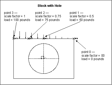
For example, the bounding edge of the following model includes an interpolated force load of 100 pounds in the negative Y direction:

In this case, the scale values are staggered such that point 3 sees 100% of the load and point 0 sees no load. The points in between see a load that is proportional with their specific scale factors, as calculated in relation to the interpolation point scale factors.

The load above has a Force Per Unit Length spatial distribution. If you apply a total load instead, Creo Simulate normalizes the load throughout the curve such that the total load applied to the curve equals the load value on the dialog box.

When applying interpolated loads, Creo Simulate works in parameter space. Parameter space is representative space, internal to the code, in which Creo Simulate represents model geometry. Creo Simulate calculates the interpolation in parameter space and then maps the interpolation back to the entity over which the interpolation is defined.

This means that the interpolated load may not be applied in exactly the way you expect. Thus, with interpolated loads, be sure to use the Review button on the Load Interpolation dialog box to verify that the load is applied as required. The review function shows the relative load magnitude at different points on the entity.

This example is one of the simplest forms of an interpolated load. Depending on how you use the scale factor in relation to interpolation point location, you can shape interpolated loads in a more complex manner.

Return to Spatial Variation.