Example—Internal Flow Simulation in Creo Simulation Live
The following example illustrates the steps required to set up and run an internal transient flow simulation study using Creo Simulation Live. In this example, water flows in through two inlets at the same velocity, and flows out through a single outlet.
To try out the example, download the sample model from here.
To run an internal flow simulation study, perform the following steps:
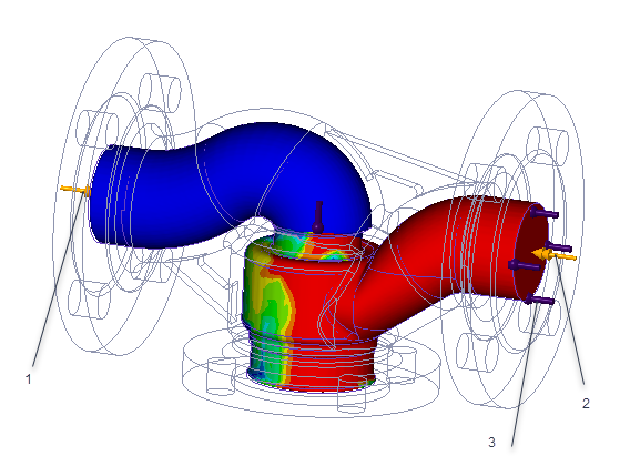
1. Open a model. In this example the model is a pipe as shown below:
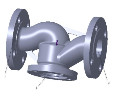
1. inlet 1
2. inlet 2
3. outlet
2. Click Live Simulation. Click >  Fluid Simulation Study. Click the arrow next to Study and select the Transient Mode check box. A fluid simulation study node with the default name Fluid1 (transient) is created and listed in the Simulation Tree.
Fluid Simulation Study. Click the arrow next to Study and select the Transient Mode check box. A fluid simulation study node with the default name Fluid1 (transient) is created and listed in the Simulation Tree.3. Click >  Internal Volume. The Internal Volume tab opens. Press CTRL and select the three bounding surfaces as shown in the following figure.
Internal Volume. The Internal Volume tab opens. Press CTRL and select the three bounding surfaces as shown in the following figure.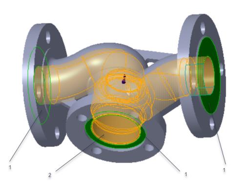
1. Bounding surfaces
2. Seed surface
The seed surfaces are automatically selected, or you can select them.
4. Click  OK to create an internal volume. The volume with the default name Internal_Volume_1 appears in the Simulation Tree.
OK to create an internal volume. The volume with the default name Internal_Volume_1 appears in the Simulation Tree.You can create an internal volume in the Creo Parametric environment or in the Creo Simulation Live environment. |
5. Right-click the fluid domain in the Simulation Tree and select Edit Materials. The Materials dialog box opens.
6. Select water.mtl from the Material Directory folder. Click OK to assign the material to the fluid domain.
7. Select the fluid inlet 1 of the model. Click Flow Velocity. The Flow Velocity dialog box opens.
8. Select Directional components to specify both magnitude and direction of velocity. Specify a value of 25 for X. Select m / sec as the value of Units. Click OK to define the inlet flow velocity.
9. Select the fluid inlet 2 of the model. Click Flow Velocity. The Flow Velocity dialog box opens.
10. Select Magnitude and direction to specify the magnitude and direction of velocity. Specify a value of -1 for X as the direction of velocity. Specify a value of 25 for Magnitude. Select m / sec as the value of Units. Click OK to define the inlet flow velocity.
11. Select the outlet surface of the model. Click Outlet Pressure. The Outlet Pressure dialog box opens. Specify a value of 0 for Magnitude, and Pa as the units. Click OK to define the outlet pressure.
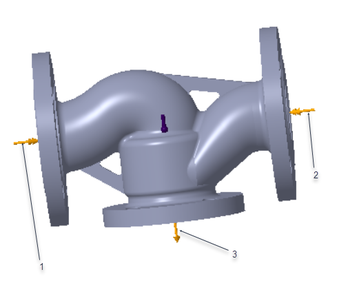
1. inlet 1 flow velocity —25 m/sec in the X- direction
2. inlet 2 flow velocity—25 m/sec in the -X- direction
3. outlet pressure —0 Pa
12. Click  Simulate to start the live simulation. The fluid flow appears in the graphics window.
Simulate to start the live simulation. The fluid flow appears in the graphics window.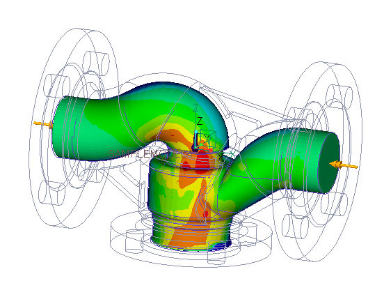
In this example the SUM component of fluid velocity is selected in the result legend. The rendering method is Surface. You can change these values to view different aspects of your results.
Effect of Thermal Boundary Conditions
For the same example, one way to model the fluid temperature is by specifying the temperature at either or both of the inlets.
1. Click > to open the Prescribed Temperature dialog box.
2. Select the inlet 2. Specify a value of 200 C as the temperature boundary condition on the selected surface. By default an initial temperature of 20 C is applied to the entire volume. You can edit this value from the Simulation Tree.
3. Select Temperature as the result quantity from the result legend with units of temperature—C. The temperature distribution within the internal volume is as shown in the following figure.
1. inlet 1 flow velocity —25 m/sec in the X- direction
2. inlet 2 flow velocity—25 m/sec in the -X- direction
3. inlet 2 temperature boundary condition — 200 C