Post-processing
There are three ways to view contours on geometric entities:
By View Tab
1. Select a boundary/ volume/ interface in the Flow Analysis Tree.
2. To display the contour, select the desired variable from Variable list under Surface group in the View Tab of Properties Panel.
By View Panel
1. Select a boundary/ volume/ interface by selecting in the Graphics Window.
2. To display the contour, select the desired variable from the  Variable option in the View Panel.
Variable option in the View Panel.By Legend
1. Select a boundary/ volume/ interface by selecting in the Graphics Window.
2. To display the contour, select the desired variable from Legend drop-down.
Create a Section
Sections, also referred to as cross-sections, are derived planar surfaces that slice through the domain or volumes at an orientation and location that you specify. Use sections to reveal features or display a Variable.
Create a section by following the steps below:
1. Click >  Flow Analysis. The Flow Analysis tab appears.
Flow Analysis. The Flow Analysis tab appears.2. Click  New Project.
New Project.3. In the Post-processing group, click  Section View. In the Flow Analysis Tree, under Derived Surfaces a new entity Section 01 is created.
Section View. In the Flow Analysis Tree, under Derived Surfaces a new entity Section 01 is created.4. Select Section 01.
5. In the Properties panel, click the Model tab.
6. Under Surface, specify the following values:
◦ Type—Plane X, Plane Y, Plane Z
◦ Position—Specify the coordinate or drag the slider to adjust the position of the section. The section can also be moved by dragging the section-normal visible in the Graphics Window.
◦ Arbitrary Plane—The normal and origin of the required plane can be specified in the dialog box.
◦ Sections created in the Creo CAD environment can be linked to CFA. For example, XSEC0001, a plane defined in Creo CAD, can be used to create Section 01 in CFA. If the Creo section XSEC0001 is modified, the associated section in CFA is automatically updated to reflect the changes.

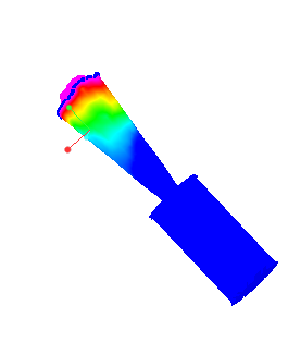
Display Grid or Contours on a Section
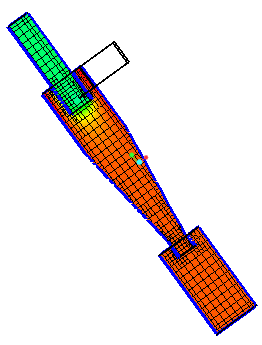 | Pressure: [Pa] : Flow 101343.937500  101313.132813 |
1. In the Flow Analysis Tree, under Derived Surfaces, select Section 01.
2. Specify the following values:
a. Surface—Yes
b. Grid—Yes
Contours for variables on a section
1. In the Flow Analysis Tree, under Derived Surfaces, select Section 01.
2. Under Surface, specify Variable—Density: [kg/m3] : Common or Cell Volume: [m3] : Common.
Monitoring Points
A point is a specified X, Y, Z coordinate within a model, used to record variables or property data at that location. The position of a point is associated with a given mesh cell based on its location at the start of a simulation. If the mesh moves, the point will move with the cell. When a point moves with the mesh, its new position is not graphically updated.
To create a monitoring point,
1. In the Post-processing group, click  Monitor Points. In the Flow Analysis Tree, under Derived Surfaces a new point Point 01 is created.
Monitor Points. In the Flow Analysis Tree, under Derived Surfaces a new point Point 01 is created.2. For Section 01, specify the Type and Position under the Properties Pane of the Model tab. The variables to be output at the point are also specified.
There are four different ways to create Points, distinguished by how their positions change during a transient simulation. They are specified under Type as follows:
• Fixed to An Initial Cell— The Point remains attached to a specified cell even if the cell is moving.
• Stationary— The Point remains at a specified location and is not affected by mesh motion.
• Prescribe Motion— Allows to specify the location of the Point using the Expression Editor, typically as a function of time.
Datum points created in the Creo CAD environment can be used as references to create monitoring points in CFA. For example, PNT0, a datum point defined in Creo CAD, can serve as a reference for a monitoring point. If the position of the datum point is modified, the corresponding monitoring point in CFA is updated automatically.

Monitor Points Distribution
Multiple equidistant monitoring points can be created by using the Monitor Points Distribution option.
To create a monitor point distribution:
• Click on the drop-down option for Monitor Points under the Post-processing group of the CFA Ribbon. In the drop-down, click on Monitor Points Distribution. The Monitor Points Distribution tab opens.
• Select the type of edge, curve or surface to be used for the distribution.
• Specify the number of points.
• Click on  to create the monitor points.
to create the monitor points.• The specified number of monitor points are added under > of the Flow Analysis Tree.
Real-time Probe
A Real-time Probe shows the value of the displayed variable on any volume, boundary or interface along with the X, Y and Z co-ordinate at the location of the mouse-pointer. To use a real-time probe, perform the following steps:
1. Display the variable on the desired volume, boundary or interface by following the steps mentioned in Contours on Volumes, Boundaries and Interfaces.
2. Select Real-time Probe from Post-Processing drop-down list.
3. Move the mouse-pointer at the desired location on the visible surfaces.
4. The variable value and co-ordinates at that location is shown in a dialog box on the bottom right corner of the screen.
Streamlines
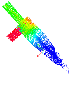 | Velocity Magnitude : [m/s] : Flow 5.969755  0.000000 |
Streamlines are used to track the path of flow. They show the direction in which a fluid element travels at any point in time. To create a streamline, complete the following steps:
1. Select Physics Module under Operations group in the CFA ribbon. The Physical Model Selection dialog box opens.
2. Select Streamline from Available Modules. Click  . The Streamline module is added under Physics in the Flow Analysis Tree.
. The Streamline module is added under Physics in the Flow Analysis Tree.3. An entity Streamline is added to the Flow Analysis Tree under Derived Surfaces.
The appearance of a given Streamline depends on the following parameters specified in the > tab:
• Line Thickness— It is used to control the thickness of streamlines and is specified in terms of absolute value (m).
• Animation Time Step Size— When set to a non-zero positive real number, together with an assignment for streamline display variable, each streamline will be divided into multiple sections and each section will keep moving along the flow direction with a speed proportional to the local flow speed. The length of a streamline section equals the local velocity times the animation time size.
• Maximum Integral Steps— It is used to limit how far the streamline algorithm will track a streamline. This prevents the Streamline module from spending excessive computation time trying to track a streamline that is either looping or near stagnant. A smaller value reduces the amount of calculations, but may end a streamline earlier than desired.
Streamlines can be enabled from a boundary or a volume:
• To enable a streamline from a boundary, complete the following steps:
a. Select a general boundary from where the streamline should begin.
b. Set Release Particle to Yes under Streamline in the > tab.
• To enable a streamline from a volume, complete the following steps:
1. Select a domain from where the streamline should begin.
2. Set Release Particle to Yes under Streamline in the > tab.
3. Click on the desired pattern under Create a New Pattern and specify the parameters of the pattern.
More details about the patterns are available in the Volume Conditions topic.
When streamlines are enabled from a volume, the Dynamic Streamlines option under Post-Processing group in the Flow Analysis Ribbon can be activated to control the position of the reference point by moving the control point in the display area.
Indicators can be added to Streamlines in the View tab of the Properties Panel. There are two types of indicators available:
• Arrow – The size of arrows can be controlled by Arrow Height and Arrow Radius.
• Sphere – The size of sphere can be controlled by Sphere Radius.
The number of indicators can be controlled by changing the Density of Indicators from coarse, normal, fine and finest.
Streamline animation is activated when Animation Time Size is increased from 0. Two additional options are available in the View tab of the Properties Panel:
• Release Mode – Streamline sections can be released either continuously from the release point using the continuous mode or as a single streamline section from each release point using the single mode.
• Relative Animation Speed – Controls the moving speed of streamline sections.
To export the streamline animation as a .gif file, follow the steps listed below after the streamline animation is activated:
1. Select the Save Streamline animation option from the Project drop-down list in the CFA Ribbon.
2. Enter the name of the file in the Save dialog box.
3. Click Save. The animation is stored in the working directory.
Isosurface
 | Velocity Magnitude: [m/s] : Flow 1.000000  0.000000 |
Isosurfaces are surfaces that envelope regions less-than (Below Value), equal-to (Single Value), or greater than (Above Value), a specified scalar value of a selected Variable, derived variable, or Property. Isosurfaces can also envelope the region between two scalars using a Value Range.
To create an isosurface, follow the steps listed below:
1. Click Flow Analysis >  Isosurface.
Flow Analysis > Isosurface.2. In the Flow Analysis Tree, a new entity Isosurface 01 appears under Derived Surfaces.
The shape of an isosurface depends on theIsosurface Variable,Type, and Value set in the Properties panel.
Legend
When coloring any display object (volume, boundary, streamline etc.) using a variable, a legend bar is associated with the variable to match the variable values to each individual color.
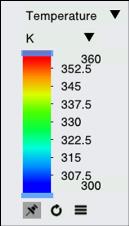
The Legend bar includes the following options:
• Variable: Select the variable from the drop-down list.
• Unit of the variable: Select the unit from the drop-down list.
• Variable Range: Drag the sliders at the top and bottom to control the maximum and minimum range of the displayed variable.
•  Refresh: Reset the range to the minimum and maximum values.
Refresh: Reset the range to the minimum and maximum values.• Following options are available under  More option:
More option:◦ Auto Refresh: When enabled, the range is refreshed as the simulation progresses.
◦ Show Values: Display the values between minimum and maximum values on the legend.
◦ Smooth Color Map: Switches between Smooth vs. Stepped color maps for surfaces. If Smooth Color Map is checked, the transition of colors over the surface is continuous, providing a smooth color map.
◦ Local Range: Resets the range to minimum and maximum values of the variable corresponding to selected geometric entities.
◦ Color Scheme: Choose between two color-schemes: Blue-red and Blue-purple.
◦ Number of Colors: Specifies the number of legend colors.
XY Plots
The quantitative results of the simulation are shown using the XY- Plots. Review the results on the boundaries or the volumes or on monitoring points, such as for mass flux, temperature, and so on.
To invoke an XY-plot, follow the steps listed below:
1. In the Flow Analysis tree, under Results, select a simulation entity (boundary, interface, volume or monitor point).
2. In the Post-processing group, click  XYPlot. A new entity xyplot1 appears under Results in the Flow Analysis Tree.
XYPlot. A new entity xyplot1 appears under Results in the Flow Analysis Tree.3. Select this entity.
4. In the Properties panel under Variable, select the variable to be plotted.
5. In the Post-processing group, click XYPlot Panel. The XYPlot Panel opens as shown below:
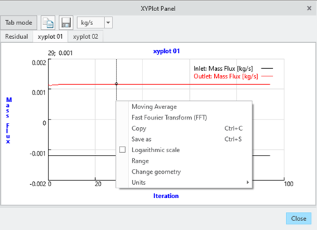
Right click in the XY Plot to access additional options:
• Moving Average: The moving average is used to obtain the average behavior over a user defined sampling interval for the entire simulation range.
• Fast Fourier Transform: This option is used to display the plot in frequency domain using Fast Fourier Transform (FFT).
• Copy: The data in the XY Plot will be copied to clipboard and can be pasted in external files like Excel, Notepad, etc.
• Save as: To save the XY Plot data as a CSV or Text file.
• Logarithmic scale: To display the data in logarithmic scale.
• Range: To specify the maximum and minimum range of X and Y values for the XY Plot.
• Change geometry: To change the selected simulation entity for the XY Plot.
• Units: To change the units of the XY Plot.
For details about output variables see Flow Output Variables, Turbulence Output Variables, Heat Output Variables.
Save Display Settings
The settings of the Display window such as model orientation and selected simulation entities in the flow analysis tree can be saved for future use. To save a scene:
1. Click Simulation Scene in the Post-processing drop-down list in the CFA Ribbon.
2. In the Simulation Scene dialog box, click New to save the scene.
To restore a saved model orientation and simulation entities selection status:
1. Click Simulation Scene in the Post-processing drop-down list in the CFA Ribbon.
2. In the Simulation Scene dialog box, select the scene from the list.
3. Click Apply to restore the saved scene.
Simulation Report
The Simulation Report Wizard enables users to create a detailed report summarizing key aspects of the current simulation, including geometry, mesh configuration, operating conditions, solver settings, and results. The generated report is saved in HTML format for easy access and sharing. To access the Simulation Report Wizard, navigate to the Project drop-down menu and select Simulation Report. The contents of the Simulation Report Wizard are outlined below:

• Model Information— This section provides an overview of the CAD model, mesh, and materials used in the fluid/solid domain.
• Physics Modules— Lists the physics modules used in the simulation and displays the user-modified solver parameters for each module.
• Working Conditions— Summarizes the user-defined boundary and volume conditions used in the simulation, along with screenshots of the boundaries.
• Mesh— Details the mesh settings used to discretize the model, presented in a tabulated form, along with grid and geometry information, including the number of cells and the model’s maximum and minimum bounds.
• Simulation Controls— Offers an overview of the simulation type (steady/transient), time definition, result-saving frequency, and the number of iterations. It also includes a residual plot of the simulation.
• Results— The user can enable post-processing options such as streamlines, particles, surface contours, plots, etc., to include them in the report. After selecting the desired items to include in the report, the corresponding tabs are activated for further customization.
Click on Finish to complete setting up the Simulation Report Wizard. Enter the name of the simulation report. Under Type, choose either Web Page to save the report in HTML format or MS PowerPoint to save the report in PowerPoint format.