Interpreting Results in Fatigue Studies
The following topic describes the different results you can define for fatigue studies with some guidance on how to interpret the results:
Biaxial Indication
Biaxial indication is a dimensionless result that shows the multiaxial nature of the stress state at a location when performing a fatigue analysis. It helps you understand whether fatigue damage is driven by one dominant principal stress or two or more principal stresses of comparable magnitude. This result helps to interpret other fatigue results like fatigue life, damage, or safety factor.
Biaxial indication measures the ratio of the smaller principal stress to the larger principal stress (excluding the principal stress closest to zero) to determine the nature of the stress state, helping to identify if fatigue life predictions (which assume uniaxial loading) are valid.
The values of biaxial indication range from -1 to 1. and can be interpreted as follows:
• -1—A value of -1 indicates pure shear. It is common in torsional loading. It requires switching from equivalent stress (von Mises) to max shear stress to obtain conservative fatigue life.
• 0—A value of 0 indicates uniaxial loading and means the stresses are pure tension or compression. Fatigue analysis assumptions are most accurate here.
• 1—A value of 1 indicates pure biaxial loading with equal tension or compression in two directions.
Use this result to verify if your model is undergoing multiaxial loading. If it is not uniaxial (0), the fatigue life results may need more careful evaluation using multiaxial fatigue criteria.
Equivalent Alternating Stress (EAS)
This is a a single stress value that represents “how damaging” your loading is for fatigue. It converts complex, multiaxial, and nonzero mean stress loading into one equivalent, fully reversed stress amplitude. This is the stress value used to read fatigue life from the S–N curve.
The EAS includes the following conversions:
• Multiaxial stress conversion—Combines stresses from different directions into one equivalent stress.
• Mean stress correction—Uses models like Goodman, Gerber, or Soderberg (not available currently but will be available in future releases) to adjust for tensile or compressive mean stress.
• Final scalar value —Directly compared with the S–N curve of the material.
The following figure shows the S-N curve and EAS. The Y- axis shows the stress amplitude (S) and the X- axis gives the cycles to failure (N).
S–N curve with Equivalent Alternating Stress
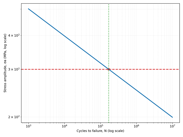
The graph shows the following values:
• Blue line: a typical S–N curve (stress amplitude vs. cycles).
• Red dashed line: the equivalent alternating stress (EAS).
• Green dotted line +red dot: the predicted life where EAS intersects the S–N curve.
You can read the graph as follows:
• Move horizontally from EAS to the S–N curve, then down to the N-axis.
• That N value is the predicted fatigue life (cycles) for the current loading.
Fatigue Damage (Miner’s Rule)
Damage = Design Life / Predicted Life.
Damage > 1 means failure before design life.
Miner’s rule damage bar
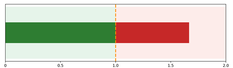
Damage D =Design Life/Predicted Life
The damage bar shows the following:
• Green area: Damage < 1—safe for design life.
• Orange dashed line at Damage = 1 —threshold.
• Red area: Damage >1—will fail before design life.
• Example shown: D = 1.67—unsafe (consumes life faster than allowed).
You can interpret the damage bar as follows:
• If the bar stops before the threshold line the design life is ok.
• If it crosses the line, expect failure before target life unless you reduce loads or redesign.
Fatigue Life
This result is the predicted number of cycles the model can survive under the given loading
This result can be interpreted as follows:
For constant amplitude loading—Value of fatigue life is the number of cycles to failure
For variable or block loading—Value of fatigue life represents number of load blocks (or equivalent cycles) to failure.
Higher life implies better fatigue performance.
Safety Factor
It is a measure of how close the component is to fatigue failure. It implies how much the load can be multiplied before fatigue failure occurs.
Safety Factor=Allowable Fatigue Strength / Applied Cyclic Stress
Safety Factor SF
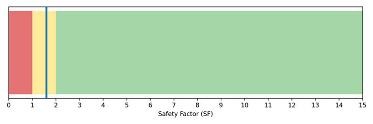
The safety factor gauge shows the following:
• Red: SF < 1—unsafe.
• Yellow: 1 ≤ SF < 2—marginal.
• Green: SF ≥ 2—comfortable margin.
• Blue marker: example SF = 1.6 —watch list; consider improvements if requirement is ≥ 2.
You can interpret the safety factor gauge as follows:
• SF < 1—Increase strength or reduce cyclic stress.
• SF ≈ 1—Component meets design life goal with a very small margin.
• SF ≫ 1—Higher margin indicates that the component is safe.
Creo Ansys Simulation limits the displayed maximum safety factor to 15 (very safe). |
Summary—Quick Reference for Fatigue Results
Result Quantity | What it Represents | How to Interpret this Result |
|---|---|---|
Equivalent Alternating Stress (EAS) | Final stress amplitude used for S–N curve lookup; Includes multiaxial + mean stress effects | Higher EAS—lower fatigue life Extremely high value—mean stress exceeded limits |
Fatigue Damage | Fraction of life consumed | Damage > 1— will fail before design life |
Fatigue Life | Predicted cycles (or blocks) until failure | Higher life = better durability |
Safety Factor | Margin against fatigue failure |
Choosing the Right Mean-Stress Correction in Fatigue Design
When defining fatigue behavior for the zero or ratio type of loading you can choose the mean stress theory to use. Selecting the correct mean-stress correction is critical because different models give different levels of conservatism. This guide helps you to pick the right mean stress theory depending on material behavior, risk acceptance, and application type.
Goodman + Gerber Diagram with Safe and Unsafe Regions
The following figure shows how the Goodman and Gerber criteria apply a mean stress correction based on the values of alternating stress and mean stress.
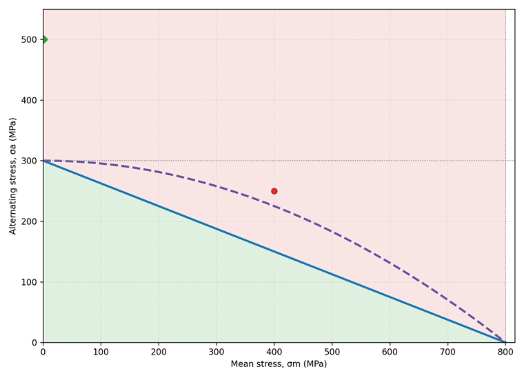
The diagram contains the following:
• Blue line represents the Goodman line (σₐ/Se + σₘ/Sut = 1).
• Dashed Parabolic Line: Gerber line σₐ = Se (1−(Sut / σₘ)2))
• Red point: your applied stress state (mean stress σₘ, alternating σₐ).
• Green arrow + green point at σₘ=0: the equivalent fully reversed amplitude (σₐ, eq) used for S–N lookup
You can interpret the diagram as follows:
• Higher mean stress (σₘ) reduces allowable alternating stress.
• The equivalent alternating stress (σₐ,eq) is what you compared to the endurance S–N curve.
The following table shows a comparison between the Goodman and Gerber mean stress theories.
Mean Stress Theory | Goodman Criteria | Gerber Criteria |
|---|---|---|
About | Moderate conservatism Widely used in industry. Use Goodman when you want a balance between safety and economy and have well-characterized loading (common for machine elements). | Least conservative Best match for ductile steel behavior. Use Gerber when the material is ductile steel with good quality control and you need lighter, optimized designs under significant tensile mean stress. |
Equation | 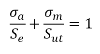 where: σa is alternating stress σm is mean stress Se is endurance limit Sut is ultimate tensile strength | 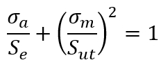 where: σa is alternating stress σm is mean stress Se is endurance limit Sut is ultimate tensile strength |
Typical Applications | • Rotating shafts • Gear teeth • Welded components • Machine elements in general • Automotive structures | • Automotive weight-optimized components • Rotating machinery designed for performance • Steel parts with strong reliability data • Non-safety-critical consumer machinery |
Pros | Simple Reasonably conservative Works well for most metals. | Best fit for experimental fatigue curves of ductile steels More realistic allowable stresses Often used in optimization/lightweight design |
Cons | Still a linear approximation (may be too conservative for ductile steels) Doesn’t match real failure behavior of ductile steels as well as Gerber | Not appropriate for brittle materials Not suitable when failure consequences are severe Not accepted in many safety-critical design codes |
Quick Decision Table
Scenario / Requirement | Best Method | Why? |
|---|---|---|
High safety / human risk | Soderberg | Prevents yielding; very conservative |
General-purpose mechanical design | Goodman | Balanced, widely accepted |
Optimized lightweight metal parts | Gerber | Best fit for ductile steel fatigue behavior |
Loads highly uncertain | Soderberg | Error margin is safer |
Known tensile mean stresses | Gerber | Parabolic curve matches steel behavior |
Regulatory approval needed | Goodman or Soderberg | Defined in most standards |
Brittle materials | Goodman | Gerber is not valid for brittle behavior |
Althought Soderberg mean stress theory is not yet available it will be in a future release and so has been included for the sake of comparison. |
Absolute No-Go Rules
• Do not use Gerber for brittle materials (cast iron, ceramics).
• Do not use Soderberg for components that must optimize weight (it can over-constrain design).
• Do not assume all criteria yield similar results; they can differ significantly near high mean stresses.