Use the polyfitc, line, slope, and intercept functions to find the least-squares line of best fit through a set of x-y data. Use the stderr function to calculate the error in fitted parameters. Calculate confidence limits around the line of best fit and form confidence intervals.
Line of Best Fit
Create a linear function to estimate how long it takes to drive various distances.
1. Define a set of distances in miles, and the time it takes in minutes, to drive these distances.
2. Define a univariate linear regression equation.
3. Call polyfitc to calculate the coefficients of regression a and b.
The coefficients are such that the difference between the values in T and the values calculated by the regression equation f is a minimum for each x value. You can check this by using a solve block and the minimize function to minimize the sum of squares:
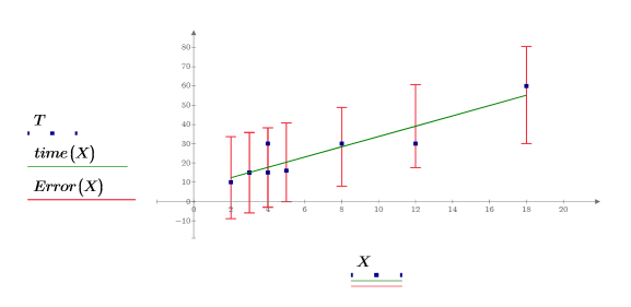
4. Define the line of best fit which minimizes the sum of the squares of the distances from each point to the line.
You should use parametrized equation from linear or any other type of regression should be used only for values near the original observed data. The line of best fit for the above data predicts that it takes the following time to travel a distance of 0 miles:
This does not make sense if the measured time is strictly travel time at constant velocity. This kind of result can sometimes represent a particular physical phenomenon. In this case, the time needed to drive zero mile may be interpreted as the average waiting time at traffic lights.
5. Plot the data points and the line of best fit.
Alternative Methods to Calculate the Slope and Intercept
There are several methods to calculate the slope and intercept for the line of best fit. For example, the line function combines the slope and intercept functions. Other methods include matrix calculations or statistical relationships.
1. Call the intercept and slope functions.
2. Call the line function.
3. Use matrix calculation by utilizing the augment function.
4. Use statistical relationships by utilizing the stdev, corr, mean and slope functions.
5. Use a plot to show that the least-squares line always passes through the (mean(X), mean(T)) point:
Standard Errors
Calculate the standard error in the estimate (also called the standard error) to measure how good the above linear fit is. Also calculate the error in the slope and in the intercept.
1. Define the degrees of freedom (the number of data points minus the number of fitted parameters).
2. Call the stderr function to calculate the standard error in the estimate for the line of best fit defined above.
This is the square root of the mean squared error, MSE, or σ2:
3. Compare the calculated standard error with the standard error returned by the polyfitstat function.
4. Calculate the standard errors in the slope and in the intercept.
5. Repeat the above calculation using matrix calculation.
6. Use the augment function to show that the standard errors for each regression coefficient are recorded in the matrix returned by the polyfitc function.
Confidence Intervals for Each Coefficient
Use the above estimates, together with percentile points from the Student's t distribution, to form a confidence interval for the estimates of the slope and the intercept.
1. Define the significance level for a 98% confidence interval and use function qt to calculate the t-factor.
2. Calculate the confidence limits for the slope.
There is a 98% chance that the actual slope value falls between SL and SU.
3. Calculate the confidence limits for the intercept.
The wide range on this value reflects the high level of scatter in the data.
4. Call the confidence function to repeat steps 1 to 3.
The confidence function returns the confidence interval widths in its first column and the t-factor in its second column. When you divide the widths by the t-factor, you get back the standard errors in both parameters:
5. To find the confidence limits, add or subtracts the width from the relevant parameter:
6. Use the augment function to show that the standard errors for each regression coefficient are recorded in the matrix returned by the polyfitc function.
Confidence Intervals for the Regression
1. Use functions length and mean to calculate a confidence interval for the regression itself.
2. Use the above function to calculate the confidence interval for any predicted x value:
3. Use matrix calculation:
4. Plot data, the line of best fit, and the confidence interval for the entire regression region.
The confidence region for predicted values has a waist near the center of the measured values. This is because the formulas used to calculate the regression are mean-based, so the values predicted closer to the mean of the data are more accurate.
5. Calculate the confidence limits on the measured values. These limits are slightly different from the limits for predicted values.
6. Use matrix calculation:
7. Plot the confidence limits as an error trace.
You can use the graphs as a form of outlier detection where measured values falling outside the confidence intervals indicate an outlier.