Boundary Conditions
The boundary condition parameters for the
Flow module apply to boundaries in the Flow Analysis Tree. The options also apply to interfaces for which the
Flow module is blanked on one side of the interface, creating a
Boundary.
The boundary conditions appear in the Properties panel when a boundary is selected in the Flow Analysis Tree under General Boundaries.
Wall
The
Wall boundary condition for
Flow corresponds to a solid boundary. Wall for the
Flow module means that there is shear (drag) and no normal component of
velocity at the boundary such as no through-flow. When the
Turbulence module is active, you can account for the roughness of the wall using the
Wall Roughness Model options. You can use options to assign a shear wall velocity to
Wall boundary conditions.
|
|
 The Wall boundary condition is the default condition for the Flow module. |
• Options
To introduce shear at the wall, select
Options for the
Wall boundary condition in the
Flow module.
◦ Stationary—Assumes that the wall is stationary.
◦ Cartesian—Introduces shear at the wall in terms of
X,
Y, and
Z components of velocity. The
velocity at a
Wall boundary condition is input relative to the stationary lab frame.
◦ Tangential—Introduces shear at the wall in terms of the normal to the wall. The tangential velocity at wall boundary conditions is input relative in terms of the Vector Normal to Wall Velocity and a value.
The
velocity for a
Wall boundary condition is intended to introduce a shear at the wall. In this instance, only tangential velocities are used.
Numerically, the velocity for a
Wall boundary condition introduces a momentum source into the
momentum. The velocity for a
Wall boundary condition does not actually move the boundary because it does not change the shape of the domain.
• Wall Type
For Wall Type, specify one of the following:
◦ Rigid—Produces a nondeforming wall.
◦ Flexible—Produces a deforming wall that does not physically move the grid associated with the wall. The effect of the wall motion is included by changing the effective volume of the neighboring cell.
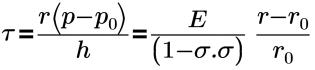
The following equation calculates the stresses and virtual displacements and wall velocity:
where,
τ | wall shear stress |
r | pipe radius |
r0 | reference radius |
p | fluid pressure(Pa) |
p0 | reference pressure |
h | wall thickness |
E | Young's modulus |
σ | Poisson ratio |
For Deformation Model, the model flexible walls are completed in two ways:
◦ Elastic Pipe model—Requires radius, wall thickness, Young’s modulus, Poisson ratio, and reference pressure as inputs, as a function of (x,y,z,t) and any valid variables. This is achieved using an analytical expression or specified using a table.
◦ User Defined—Specifies the displacement as a function of pressure using an analytical expression or in tabular form.
• High Order Shear
The
High Order Shear option for the
Wall boundary condition in the
Flow module uses a parabolic function for the velocity profile near the wall instead of a linear function. You can use this function in the following cases:
◦ For laminar flow near the wall
◦ If the near wall cell is within the laminar sublayer for turbulent flows
◦ To reduce the number of cells used to resolve flow within thin gaps which are heavily dominated by viscous shear forces.
Specified Velocity
Use
Specified Velocity boundary condition to set the fluid
velocity (m/s) at an opening, creating an inlet, outlet, or combination of both.
Specified Velocity sets the velocity on the boundary. The corresponding mass flow is accordingly determined by the fluid density and velocity, relative to the boundary area and orientation. You can set the direction and magnitude of the velocity for the
Specified Velocity boundary condition using the options described below:
• Cartesian—Input the boundary velocity in terms of the X, Y, and Z velocity components relative to the model coordinate system.
• Boundary Normal—Input the boundary velocity normal to the boundary. The magnitude is controlled by the Normal Velocity Component. The flow direction is set by selecting Inflow, Outflow, or Both:
◦ Inflow—Allows flow into the domain.
◦ Outflow—Allows flow out of the domain.
◦ Both—Allows flow in or out of the domain.
For either Inflow or Outflow, a negative Normal Velocity Component is reset to a positive value, such that the sign of the value for the volumetric flux has no influence on the direction of flow.
| In Creo Flow Analysis, a positive mass flux or volumetric flux at a Boundary corresponds to outflow. |
• Swirl—Introduces a swirling flow at a Boundary. The magnitude of the inflow is controlled by the Normal Velocity Component. The flow direction is set by selecting Inflow, Outflow, or Both. The swirl velocity is controlled by the: Rotational Speed, Rotational Center, and Rotational Axis Vector.
◦ The direction of the rotation of a swirl is specified relative to the stationary (lab) frame of reference, from the perspective of an observer with the rotational axis vector aimed straight on. Rotational direction of clockwise or counterclockwise only accepts a positive value of rotational speed. If you select both for the direction of the rotation of a swirl, you can specify the direction of rotation based on the sign of the rotational speed, such that positive produces a clockwise rotation and negative implies counterclockwise.
◦ The magnitude of the rotational speed of a boundary is specified relative to the stationary (lab) frame of reference.
Specified Volumetric Flux
Use
Specified Volumetric Flux boundary condition to set the volumetric flux (m
3/s) of the fluid, creating an inlet, outlet, or a combination of both.
Specified Volumetric Flux sets the velocity on the boundary. The corresponding mass flow is accordingly determined by the fluid density ρ and velocity v, relative to the boundary area and orientation. The
Specified Volumetric Flux refers to the integral of the volumetric fluxes over the boundary. The velocity associated with a
Specified Volumetric Flux can be
Uniform or based on a
Fully Developed. You can specify the direction and magnitude of the
velocity using the following options:
1. Flow Direction—Controlled by selecting Inflow, Outflow, or Both.
2. Velocity Profile—Set the velocity profile for the Specified Volumetric Flux boundary condition to one of the following:
◦ Uniform—Constant velocity at the boundary based on the boundary area (A) and orientation: V = (Volumetric Flux)/Area.
◦ Fully Developed—Velocity profile at the boundary is similar (same shape) to the velocity profile at the cell centers immediately downstream.
Specified Total Pressure
Use Specified Total Pressure boundary condition to set the Total Pressure at an opening where flow is expected to enter or leave the domain. The velocity of the flow at the boundary is then computed as part of the solution. You can specify direction and pressure.
• Directional Option—Direction of the boundary velocity vector is constrained using the following options:
◦ Cartesian—Constrains the boundary velocity to be in a specified direction, relative to the model coordinate system. The Flow Direction vector components (X, Y, and Z) are used in conjunction with the Cartesian option to constrain the boundary velocity to a specified direction.
◦ Boundary Normal—Constrains the boundary velocity to be normal to the boundary. Boundary Normal uses the local normal of each cell face in the selected boundary.
• Total Pressure
• Velocity Profile—Sets the velocity profile for the Specified Volumetric Flux boundary condition to one of the following:
◦ Uniform—Constant total pressure at the boundary based on the Boundary area (A) and orientation.
◦ Zero Gradient—Total pressure at the boundary based on an extrapolation of the interior total pressures. There is no change or no gradient.
Rotating Wall
The Rotating Wall simulates the shear effect of a rotating wall. It has the following options:
• Wall Type—Specify Rigid or Flexible
• High Order Shear
• Rotational Direction—Determines the direction of rotation for a rotating wall. The direction of a boundary rotation is specified relative to the stationary (lab) frame of reference, from the perspective of an observer with the rotational axis vector aimed straight on. Select Both Directions of the rotation of a boundary to specify the direction of rotation. This direction is based on the sign of the rotational speed, such that positive produces a clockwise rotation and negative implies counterclockwise.
• Rotational Speed
• Rotational Axis Vector
• Rotational Center
• Axial Velocity
• Output
Symmetry
Symmetry for flow means that there is no shear (that is perfect slip) and no normal component of velocity at the boundary (that is no through-flow). Symmetry for flow also means there is no normal gradient of pressure at the boundary. Symmetry for flow is different than the wall boundary conditions in that for a wall there is shear. A Symmetry boundary condition for flow usually corresponds to a physical symmetry in the model. It does not have to, however, if the effects of this boundary condition are logical. For example, you can use this to mimic a free surface.
The integrated quantities available as output from the
Symmetry boundary condition are
Area and
Normal.
Specified Pressure Outlet
Use Specified Pressure Outlet boundary condition to set the static pressure at an opening where flow is expected to exit the domain. In case of back flow, a momentum source can also be added by the associated Back Flow Velocity(optional) and its (X, Y, Z) input. Specified pressure outlet determines the mass flow across the boundary as part of the solution.
Specified Pressure Outlet boundary condition contains the following options:
• Pressure—Determines the
Static Pressure at the outlet. If the properties of the fluid depend on the pressure, then pressure should be the absolute pressure. Otherwise, it can be a relative pressure such as gauge.
• Velocity Profile—Sets the velocity profile for the Specified Pressure Outlet boundary condition to one of the following:
◦ User Specified—Specifies a back flow velocity. Use the Back Flow Velocity(optional) parameter associated with Specified Pressure Outlet to include a momentum source for any back flow at this boundary. The values are input in terms of the X, Y, and Z components of the velocity. The Back Flow Velocity(optional) parameter does not directly affect the mass flow. It adds or subtracts momentum sources to any fluid flowing back into the domain. Flow can enter or exit the domain at a specified pressure outlet. If flow exits the domain at a specified pressure outlet (as expected), the value of Back Flow Velocity(optional) has no effect. The optional Back Flow Velocity(optional) is important if the incoming fluid has a relatively high dynamic head.
◦ Uniform—Velocity at the outlet is uniform.
◦ Fully Developed—Velocity profile at the boundary is similar (same shape) to the velocity profile at the cell centers immediately downstream.
• Output
Specified Pressure Inlet
Use Specified Pressure Inlet boundary condition to set the static pressure at an opening where flow can enter the domain. You can also add a momentum source at this type of boundary using the associated velocity input. Specified Pressure Inlet determines the mass flow across the boundary as part of the solution and contains the following options:
• Pressure—Controls the
Static Pressure at the inlet. You can include the effects of the dynamic pressure using the optional
Velocity(optional). If the incoming fluid has a relatively high dynamic head, use the
Specified Total Pressure boundary condition instead of specified pressure inlet.
• Velocity Profile—Can be specified as User Specified, Uniform, or Fully Developed.
◦ User Specified—Specifies a back flow velocity. Use the Velocity(optional) parameter associated with Specified Pressure Inlet to include a momentum source for any fluid flowing in at this boundary. The values are input in terms of the X, Y, and Z components of the velocity. The optional Velocity(optional) parameter does not directly affect the mass flow, and only adds or subtracts momentum sources to the fluid entering fluid. Flow can enter or exit the domain at a specified pressure inlet. If flow exits the domain at a specified pressure inlet, the values of the optional Velocity(optional) have no effect. The optional Velocity(optional) is important if the incoming fluid has a relatively high dynamic head.
◦ Uniform—Velocity at the inlet is uniform.
◦ Fully Developed—Velocity profile at the boundary is similar (same shape) to the velocity profile at the cell centers immediately downstream.
| If the incoming fluid has a relatively high dynamic head, you can also use the Specified Total Pressure boundary condition instead of Specified Pressure Inlet. |
Resistor Capacitor
Resistor Capacitor enables you to select from a variety of 1-D models to determine the flow-pressure relationship for a selected boundary. Mass flux (kg/s) leaving the domain has a positive value. The following models are available under Model option under Resistor Capacitor:
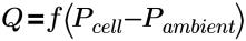
• DP-Q Curve—Specifies the flowrate as a function of pressure.
where,
Q | volumetric flux (m3 /s) |
Pambient | environment pressure (Pa) |
dP | (Pcell – Pambient) is computed and available as a local expression editor variable |
The DP-Q Curve option requires an expression or table defining the flowrate Q as a function of the Delta P (dP) for the Volumetric Flux input field. Otherwise there is no delta pressure (dP) dependence. dP as a function of the Environment Pressure and the boundary cell pressure is computed by the code and available as a local expression editor. The unit of dP is Pascal.
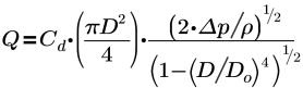
• Orifice—Computes the volumetric flow as if there were a circular orifice in the boundary. The equation and inputs are as follows:
where,
Q | volumetric flux (m3 /s) |
Δp | (Psystem – environment pressure) (Pa) |
ρ | upstream cell fluid density (kg/m3) |
D | orifice diameter (m) |
Do | diameter of upstream wall surrounding the orifice (assumed >> D, such that (D/Do)4 may be ignored). |
Ref: Frank M. White, Viscous Fluid Flow, 1974 ISBN 0-07-069710-8, p. 227 |
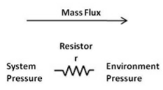
• Resistor—Computes the volumetric flow across a boundary based on the pressure drop and an effective resistance. The equation and inputs are as follows:
where,
Q | volumetric flux (m3 /s) |
Δp | Psystem – environment pressure (Pa) |
r | Resistor-r (Pa-s/m3) |
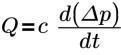
• Capacitor—Computes the volumetric flow across a boundary based on the pressure drop and a capacitance.
• 2 Elements—Determines the flow-pressure relationship for a selected Boundary based on a circuit consisting of a resistor and a capacitor. The equation for the 2 Element Resistor-Capacitor is as follows:
where,
Q | volumetric flow rate (m3 /s) |
ΔP | system pressure – environmental pressure (Pa) |
R | Resistor-R (Pa-s/m3 ) |
C | capacitor (m3/Pa) |
| This boundary condition is based on the 2-element Windkessel model used for heart flow modeling. Refs. 1) Daniel R. Kerner, Ph.D. and 2) Broemser, Ph., et. al.,``Uber die Messung des Schlagvolumens des Herzens auf unblutigem Weg'', Zeitung für Biologie 90 (1930) 467-507. |
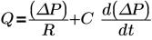
• 3 Elements—Specifies the flow-pressure relationship for a selected Boundary based on a circuit consisting of two resistors and one capacitor. The equation for the 3 Element Resistor-Capacitor is as follows:
where,
I | volumetric flow rate (m3 /s) |
ΔP | system pressure – environmental pressure |
r | Resistor-r (Pa-s/m3) |
R | Resistor-R (Pa-s/m3) |
C | Capacitor (m3/Pa) |
Mass flux (kg/s) leaving the domain has a positive value.
| This boundary condition is based on the 3-element Windkessel model often used for heart flow modeling. Refs. 1) Daniel R. Kerner, Ph.D. and 2) Broemser, Ph., et. al., ``Uber die Messung des Schlagvolumens des Herzens auf unblutigem Weg'', Zeitung für Biologie 90 (1930) 467-507. |
Interface Condition
The interface condition for the
Flow module is the same as for the boundary conditions, only if one side of the interface is
Blanked for flow. If the
Flow module is active on both sides of an
Interface, it can only be assigned as a
Default Interface.
Default Interface is the default
Flow module option for an interface connecting fluid to fluid. The
Flow module
Output available with the
Default Interface includes area, normal, mass flow rate, volumetric flow rate, momentum, pressure force, average total pressure, pressure, and average static pressure.
You can specify the following interface conditions and associated
Flow parameters for a selected
Interface under the
Flow module in the Properties panel.
• Fan—By specifying the Flow Direction, DP-Q Curve for flow-pressure relationship and Swirl (specified using Center, Tangential Velocity and Radial Velocity).
• Pressure Jump—By specifying the Flow Direction, DP-Q Curve for flow-pressure relationship and Swirl (specified using Center, Tangential Velocity and Radial Velocity).
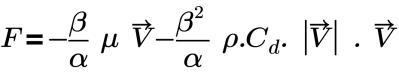
• Porous Surface—Enables the addition of a resistance due to a permeable Interface connecting fluid to fluid. The variables associated with the Surface Porous model are:Thickness, Permeability, and Quadratic Coefficient. The pressure drop per unit distance across the Interface is computed using the Darcy-Forchheimer Law:
The pressure drop across the Interface is computed by multiplying F by some finite thickness. The Porosity is set in the Common module.
Output
The integrated quantities available as output from the
Flow module for the
Boundaries appear in
output variables.