Example: Thermal Simulation
Example: Steady-State Thermal Analysis
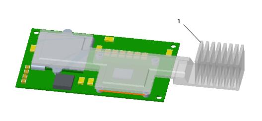
The following example demonstrates how you can use live simulation to study the effects of heat loads on a printed circuit board (PCB).
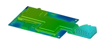
Heat loads are applied to the different groups of integrated circuits on the PCB. Boundary conditions are defined for the heat shield, one of the corner holes of the PCB and the fins of the heat shield.
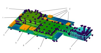
1. Heat Flow Load 1—10,000 mW
2. Heat Flow Load 2—500 mW
3. Heat Flow Load 3—50 mW
4. Heat Flow Load 4—7500 mW
5. Heat Flow Load 5–150 mW
6. Boundary Condition 1—A convection coefficient of 0.01 mW/mm2 C applied to the heat shield with an ambient temperature of 25 degree C
7. Boundary Condition 2—A prescribed temperature of 5 degree C applied to the corner hole of the PCB
8. Boundary Condition 3–A convection coefficient of 0.01 mW/mm2 C applied to the fins of the heat sink with an ambient temperature of 25 degree C
Note that result values change depending on the setting of Simulation Quality. In this example the Simulation Quality slider has a maximum (100%) value of accuracy.
When you click  Simulate the temperature results for the PCB are displayed as a fringe plot on the model in the graphics window. In this example the maximum temperature is around 199 C.
Simulate the temperature results for the PCB are displayed as a fringe plot on the model in the graphics window. In this example the maximum temperature is around 199 C.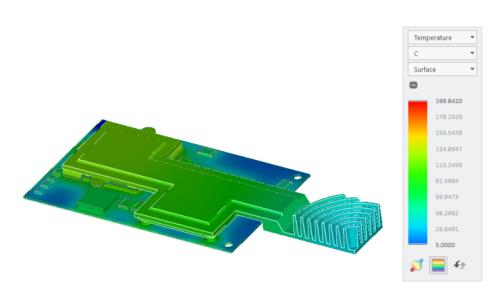
Click  to view the location on the PCB with the maximum and minimum temperature values. In this example Max Value is the selected rendering method and shows the maximum value, that is on the lower surface of the board.
to view the location on the PCB with the maximum and minimum temperature values. In this example Max Value is the selected rendering method and shows the maximum value, that is on the lower surface of the board.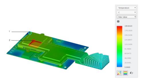
1. Minimum temperature represented by a blue circle
2. Maximum temperature represented by a red circle
To reduce the overall temperature of the model you can modify the design. In the following figure the shape of the fins of the heat shield has been changed and the height of the fins has also been increased for improved heat dissipation.
1. Modified fin shape and height of the heat shield
Click Simulate to run the thermal simulation with the new design. The results are now close to 162 C.
Simulate to run the thermal simulation with the new design. The results are now close to 162 C.
Example: Transient Thermal Analyses
For the same model with the modified fins, you can also run a transient thermal study and view temperature results at different time points.
Click the arrow next to > and select the Transient Thermal check box. Click Simulate to start the transient thermal simulation. A changing fringe plot displays as the simulation runs. Click  Pause Simulation if you want to pause the simulation.
Simulate to start the transient thermal simulation. A changing fringe plot displays as the simulation runs. Click Pause Simulation if you want to pause the simulation.When the simulation run completes the Pause Simulation button is inactive, and a message in the status bar at the bottom of the screen indicates that the simulation study run is complete. The results are similar to those of a steady-state simulation study with the same boundary conditions, loads, and geometry. The simulation time indicates the time taken for the run.
Pause Simulation button is inactive, and a message in the status bar at the bottom of the screen indicates that the simulation study run is complete. The results are similar to those of a steady-state simulation study with the same boundary conditions, loads, and geometry. The simulation time indicates the time taken for the run.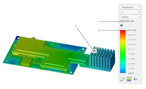
1. Simulation time for transient thermal study
2. Maximum temperature
3. Probe at point on innermost fin
Based on the completed run you can create a probe to view the temperature value at different locations on the model at the end of different simulation time. Perform the following steps:
1. Click  Simulation Probe to open the Simulation Probe dialog box.
Simulation Probe to open the Simulation Probe dialog box.2. Select a point on the innermost fin.
3. Select On Point from the Type list.
4. Click Save to save the probe.
5. Click  to view time-dependent graphs of temperature at the point for different values of simulation end time.
to view time-dependent graphs of temperature at the point for different values of simulation end time.Run transient thermal studies with different values of Simulation End Time. The following table shows the temperature results at the probed point, after setting time limits with 500 second increments.
Simulation End Time | Temperature Results at the End of Simulation Time | Temperature Chart at Point on Fin |
|---|---|---|
500 sec | 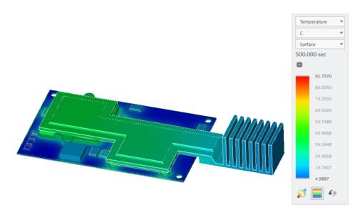 |  |
1000 sec | 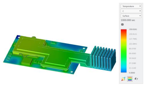 | 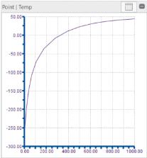 |
1500 sec | 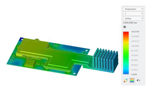 | 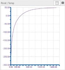 |
2000 sec | 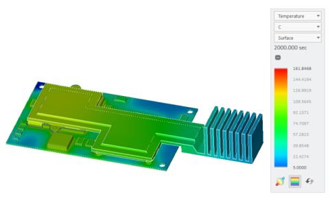 | 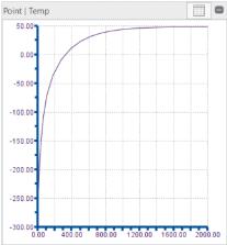 |
2500 sec | 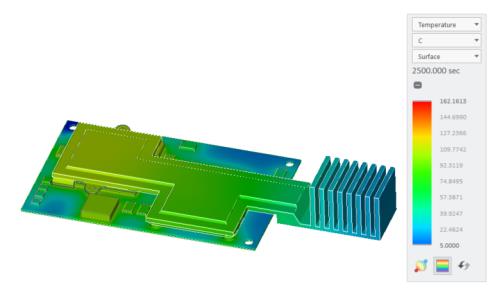 | 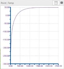 |
As seen in the graphs the temperature results attain a steady-state after 1500 seconds and are approximately the same as those of a steady-state thermal study.